
This post we will explore a type of normalizing flow called **Inverse Autoregressive Flow**. A composition (flow) of transformations, while preserving the constraints of a probability distribution (normalizing), can help us obtain highly correlated variational distributions.
Don’t repeat yourself
If what was mentioned in the previous lines didn’t ring a bell, do first read these posts: variational inference and normalizing flows. This post could really be seen as an extension of the latter.
1. Planar/ Radial flows
Rezende & Mohammed[1] discussed two normalizing flows, the planar flow, and the radial flow. If we take a look at the definition of the planar flow transformation:
\begin{equation} f(z) = z + u h(w^Tz + b) \end{equation}
Where the latent variable $z \in \mathbb{R}^D$, and the transformations learnable parameters; $u \in \mathbb{R}^D, w \in \mathbb{R}^D, b \in \mathbb{R}$, and $h(\cdot)$ is a smooth activation function.
As $w^Tz \mapsto \mathbb{R}^1$, the transformation is comparable to a neural network layer with one activation node. Evidently, this is quite restrictive and we need a lot of transformations to be able to transform high dimensional space. This same restriction is true of the radial flow variant.
2. Improving normalizing flows
As discussed in the post normalizing flows, a normalizing flow is defined as:
\begin{eqnarray} Q(z’) &=& Q(z) \left| \det \frac{\partial{f}}{\partial{z}} \right|^{-1} \end{eqnarray}
Where $f(\cdot)$ is an invertible transformation $f: \mathbb{R}^m \mapsto \mathbb{R}^m$. To have a tractable distribution, the determinant Jacobian $\left| \det \frac{\partial{f}}{\partial{z}} \right|$ should be cheaply computable.
This tractability constraint isn’t easily met, and therefore there is now a field of research that focusses on transformations $f(\cdot)$ that have tractable determinant Jacobians. With radial/ planar flows tractability is achieved by applying the matrix determinant lemma.
2.2 Autoregression
Autoregressive functions do have tractable determinant jacobians. Let $z’$ be our transformed random variable $f(z) = z’$. An autoregressive function would transform every dimension $i$ by:
\begin{eqnarray} z’_i = f(z_{1:i}) \end{eqnarray}
The Jacobian matrix $J = \frac{\partial{z’}}{\partial{z}}$ will then be lower triangular. Which is cheaply computed by the product of the diagonal values:
\begin{eqnarray} \det J = \prod_{i=1}^D J_{ii} \end{eqnarray}
Tractable determinant Jacobians are thus possible by using autoregressive transformations. The first time I read this paper[3], I wondered how we could ensure a neural network would be an autoregressive transformation without using RNNs. It turns out you can mask the connection of an autoencoder in such a way that that the output $x_i$ is only connected to the previous inputs $x_{i:k}$. This was shown in the MADE[4] paper, which was the topic of my previous post Distribution estimation with Masked Autoencoders.
Note: In the MADE post we modeled $x_i = f(x_{1:i-1})$, which would lead to a lower triangular Jacobian with zeros on the diagonal, and thus leading to $\det J = 0$. Later in this post we’ll see that this won’t be a problem.
2.3 Autoregressive transformation
The radial/ planar transformations are effectively a single layer with one activation node. The relations between different dimensions of $z$ can therefore not be very complex. With autoregressive transformations we can model more complexity as $z_i$ is dependent on $z_{1:i-1}$, and thus connected to all lower dimensions of $i$. Let’s define such a transformation. Let $z’ = f(z)$, and the first dimensions of the transformed variable be defined by:
\begin{eqnarray} z &\sim& \mathcal{N}(0, I) &\qquad \tiny{\text{base distribution: } Q(z) } \\ z’_0 &=& \mu_0 + \sigma_0 \odot z_0 \label{art0} \end{eqnarray}
Where $\epsilon \in \mathbb{R}^D$. Effectively meaning that the first dimension of the transformation is randomly sampled. The other dimensions $i \gt 0$ are computed by:
Eq. \eqref{art} clearly depicts the downside of this transformation. Applying the transformation has a complexity of $\mathcal{O}(D)$ (without any possibility to parallelize). Which can become rather expensive as we will apply a flow of $k$ transformations. Actually sampling from this distribution would be proportional to $D \times k$ operations.
2.4 Inverse Autoregressive Transformation
We can inverse the operations defined in eq. \eqref{art0} and eq. \eqref{art}.
Note that due to the inversion $z’ = f(z)$ now is $z = f(z’)$!
The inverse is only dependant on $z’$ (in this case, the value before the transformation), and can thus easily be parallelized. Besides cheap sampling, we also need to derive the determinant Jacobian. The Jacobian lower triangular, which means we only need to compute the partial derivatives of the diagonal to compute the determinant.
The diagonal is $\{{ \frac{z_0}{z’_0}, \frac{z_1}{z’_1}, \dots, \frac{z_D}{z’_D } \}}$.
As $\mu(\cdot)$ and $\sigma(\cdot)$ are not dependant of $z’_i$ (but only on $z_{1:i-1}$), the partial derivatives evaluate to $ \{{ \frac{1}{\sigma_0}, \frac{1}{\sigma_1(z’_1)}, \dots, \frac{1} {\sigma_D(z’_{1:D-1}) } \}}$ , and thus we also have a tractable determinant Jacobian;
3. Inverse Autoregressive Flow
That wraps all the ingredients we need to build a tractable flow. We will use the inverse functions defined in eq. $\eqref{iart0}$ and eq. $\eqref{iart}$. Let $t$ be one of $k$ flows. Instead of modeling $\mu_t(\cdot)$ and $\sigma_t(\cdot)$ directly, we will define two functions ${\bf s}_t = \frac{1}{\sigma_t(\cdot)}$, and ${\bf m}_t = \frac{-\mu_t(\cdot)}{\sigma_t(\cdot)}$. These will be modeled by autoregressive neural networks.
3.2 Hidden context and numerical stability
The authors[3] also discuss a hidden input $h$ for the autoregressive models, $[{\bf s}_t, {\bf m}_t ]$.
\begin{equation} [{\bf s}_t, {\bf m}_t ] \leftarrow \text{autoregressiveNN}[t]({\bf z}_t,{\bf h}; {\bf \theta}) \end{equation}
And finally for numerical stability they modify eq. \eqref{upd}, by an update rule inspired by LSTM gates.
Note that I deliberately chose $g_t$ instead of $\sigma_t$, as the authors do, so that it can’t be confused with the $\sigma(\cdot)$ defined earlier.
Let’s convince ourselves that this modification of eq. \eqref{upd} is allowed. It doesn’t break the autoregressive nature of the transformation. Therefore the Jacobian $\frac{d{\bf z_t}}{d{\bf z_{t-1}}}$ is still lower triangular. The determinant Jacobian is defined by the product of the diagonal Jacobian:
Note that ${\bf m}_t$ is not dependent of $z_{t-1,i}$ only on $z_{t,1:i-1}$ and therefore is not a term in the partial derivative.
Now we really have defined everything needed for variational inference. Eq. \eqref{transf} will be the transformation we apply, and eq. \eqref{logdet} is the final log determinant Jacobian used in the variational free energy $\mathcal{F(x)} $;
For a derivation of the variational free energy see the normalizing flows post.
Pytorch implementation & results
Below I’ve shown a code snippet of a working implementation in Pytorch. The full working exhample is hosted on github.
class AutoRegressiveNN(MADE):
    def __init__(self, in_features, hidden_features, context_features):
        super().__init__(in_features, hidden_features)
        self.context = nn.Linear(context_features, in_features)
        # remove MADE output layer
        del self.layers[len(self.layers) - 1]

    def forward(self, z, h):
        return self.layers(z) + self.context(h)


class IAF(KL_Layer):
    def __init__(self, size=1, context_size=1, auto_regressive_hidden=1):
        super().__init__()
        self.context_size = context_size
        self.s_t = AutoRegressiveNN(
            in_features=size,
            hidden_features=auto_regressive_hidden,
            context_features=context_size,
        )
        self.m_t = AutoRegressiveNN(
            in_features=size,
            hidden_features=auto_regressive_hidden,
            context_features=context_size,
        )

    def determine_log_det_jac(self, g_t):
        return torch.log(g_t + 1e-6).sum(1)

    def forward(self, z, h=None):
        if h is None:
            h = torch.zeros(self.context_size)

        # Initially s_t should be large, i.e. 1 or 2.
        s_t = self.s_t(z, h) + 1.5
        g_t = F.sigmoid(s_t)
        m_t = self.m_t(z, h)

        # log |det Jac|
        self._kl_divergence_ += self.determine_log_det_jac(g_t)

        # transformation
        return g_t * z + (1 - g_t) * m_t
I’ve trained a normalizing flow on a target distribution in 2D. The base distribution was a factorized unit Gaussian $\mathcal{N}(0, I)$. This distribution was transformed 4 times, as the examples were run with 4 flow layers. The prior distribution was also is uniform over the whole domain.
The first figure shows the Inverse Autoregressive flow. The second figure shows the Planar flow.
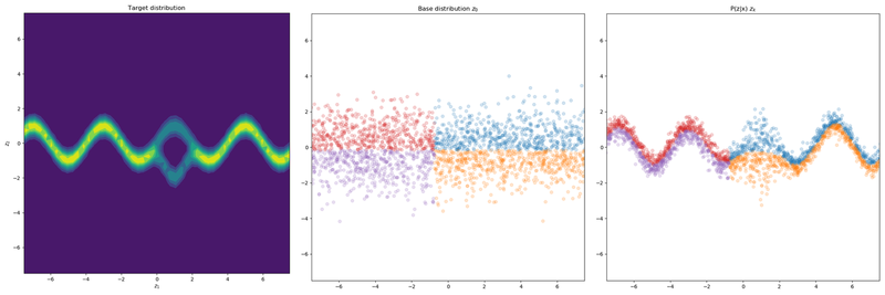
4 IAF layers
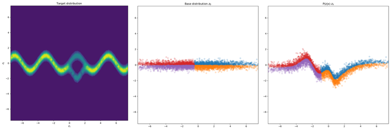
4 Planar layers
We see that the IAF layers are able to model the posterior $P(Z|X)$ better as well as stay closer to the prior $P(Z)$. The base distribution is less flattened and is a bit more uniform (though not on the whole domain). By observing that the base distribution is less modified we can conclude that normalizing flow is more powerful and is better able to morph the base distribution in the required density.
This is also visible in the figure below. This is a result from the original authors. They trained a VAE on a toy dataset with 4 data points. What we see is that the VAE with IAF layers has a base distribution that is more true to a unit Gaussian.
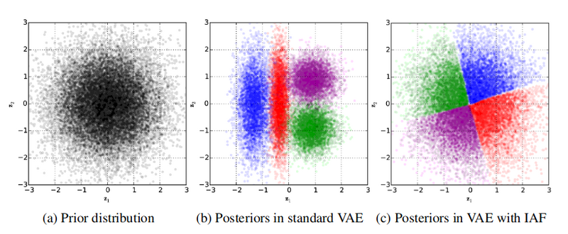
Prior and Base distributions. $^{[3]}$
Conclusion
And that’s a wrap! Another post on normalizing flows. This field of research seems really promising. But as we have seen this post, coming up with new normalizing flows isn’t easy. Here the authors were able to do so because they made two clever observations;
- Autoregressive transformation lead to simple determinant Jacobians i.e. invertible transformations
- The inverse of an autoregressive operation isn’t expensive in sampling.
If you want to read more about different types of normalizing flows out there, I’d recommend taking a look at this blog post.
References
[1] Rezende & Mohammed (2016, Jun 14) Variational Inference with Normalizing Flows. Retrieved from https://arxiv.org/pdf/1505.05770.pdf
[2] Adam Kosiorek (2018, Apr 3) Normalizing Flows. Retrieved from http://akosiorek.github.io/ml/2018/04/03/norm_flows.html
[3] Kingma, Salimans, Jozefowicz, Chen, Sutskever, & Welling (2016, Jun 15) Improving Variational Inference with Inverse Autoregressive Flow. Retrieved from https://arxiv.org/abs/1606.04934
[4] Germain, Gregor & Larochelle (2015, Feb 12) MADE: Masked Autoencoder for Distribution Estimation. Retrieved from https://arxiv.org/abs/1502.03509