
Four of my last five blog posts were more or less related to Baysian inference with variational methods. I had some momentum, and I wanted to use the traction I gained to do another post (which will come!) on enhancing variational methods with Inverse Autoregressive Flows (IAF), but first I have to get something different out of the way.
In the paper describing IAF, they refer to an autoregressive neural network (and further assume his to be clear knowlegde). Besides that I now needed to research autoregressive neural networks in order to fully understand the IAF paper, it also triggered my interest without being a roadblock. And, as it turns out, they turn to be a quite simple, but really cool on standard autoencoders. This post we will take a look at autoregressive neural networks implemented as masked autoencoders.
1. Default autoencoders
Default autoencoder try to reconstruct their input while we as algorithm designers try to prevent them from doing so (a little bit). They must a feel bit like the bullied robot in the video below. We give them a task, but also hinder the robot in doing so.
Obviously we put the autoencoders of balance by shoving them with a hockey stick. Our hindrance is more subtle. We give them a task, but we don’t provide them the required tools for executing that task. When building a shed with only have a hammer and three nails at you disposition, you have to be really creative.
The figurative nails and hammer are called a bottleneck, often named $z$, and this a narrow layer in the middle of the network. A bit more formally, let $x \in \mathbb{R}^D$, then $z \in R^{<D}$. The autoencoder consists of two parts. The encoder; $f(x) = z$, and the decoder $g(z) = x$.
The figure below shows a visual representation of an autoencoder. Where the $z$ is the latent space representation.
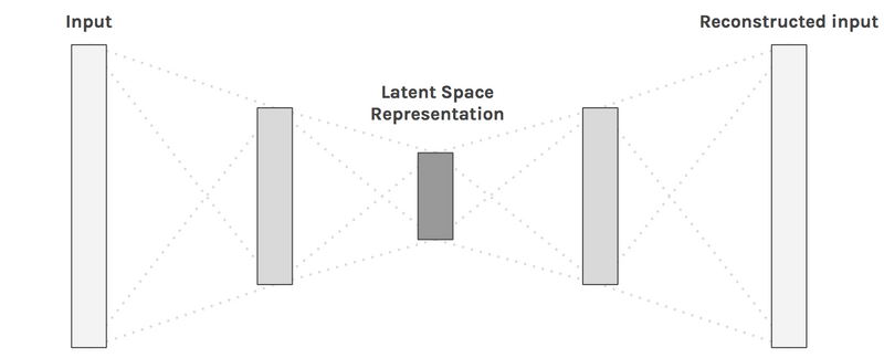
Autoencoder architecture [1].
By reducing the latent dimension, we enforce the autoencoder to map the input to a lower dimension, whilst retaining as much of the information a possible. This for instance help in:
- Denoising images (The lower dimension of $z$ filters the noise).
- Compress data (Only call the encoder $f(x)$).
2. Distribution estimation
If we bully the autoencoders just a bit more, by also blinding them partially, we can actually make them learn $P(x)$, i.e. the distribution of $x$. Germain, Gregor & Larochelle $^{[2]}$, posted their findings in the paper MADE: Masked Autoencoder for Density Estimation. In my opion, they made a really elegant observation that, by the definition of the chain rule of probability, we can learn $P(x)$ by blinding (masking) an autoencoder. Let’s explore their observation.
The chain rule of probability states:
\begin{eqnarray} P(A,B) = P(A|B) \cdot P(B) \end{eqnarray}
Which for a whole vector of $x$ is defined by:
So by learning an autoregressive relationship, we actually model the probability distribution of $x$. That’s really cool, and actually quite simple to implement! This is where the bullying of the autoencoder comes into play. All we need to do is to restrict autoencoders connections in such a way that node for predicting $x_t$, is only connected to the inputs $x_{1:t-1}$.
This principle of restricted connections is shown in the figure below for the red output $P(x_2|x_1)$. Please take a look good at it and appreciate what you see, because it took me forever to draw!
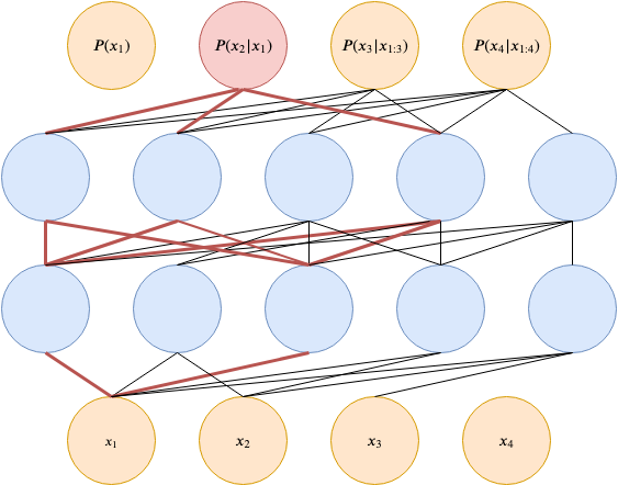
Autoregressive autoencoder [3].
3. Masking trick
The autoregressive properties of such a network are obvious, however the implementation doesn’t seem trivial at first sight. In the figure, the autoencoder is drawn with reduced connections. This isn’t how we are going to implement it however. Just as done with dropout$^{[4]}$, we nullify weight outputs by element-wise multiplying them with a binary masking matrix. Connections multiplied by one are unharmed. Connections multiplied by zero are effectually discarded. A standard neural networks layer is defined by $g(Wx + b)$, where $W$ is a weight matrix, $b$ is a bias vector, and $g$ is a non linear function. With masked autoencoders, the layer activation will become $g((W \odot M)x + b)$, where $M \in \{0, 1\}$ is the masking matrix.
3.1 Hidden nodes
For the creation of the masks, we use a clever trick. We assign a random variable $m’ \in \{1, 2, \dots, D-1 \}$ to every hidden node $k$ in the network.
Let the value of $m’$ at node $k$ and layer $l$ be $m^l(k) = m’_k $. The masking values $M_{k, k’}$ for node $k’$ connected to node $k$ (of the previous layer) are defined by:
Where $1_{m^l(k’) \ge m^{l-1}(k)}$ is the indicator function, returning $1$ if the expression is true and retuning $0$ otherwise.
3.2 Output nodes
For the output nodes of the neural network, the condition slightly changes. Let $d$ be the ouput node. The masking values are then defined by:
Note that $\ge$ becomes $\gt$. This is important as we need to shift the connections by one. The first output $x_1$ may not be connected to any nodes as it is not conditioned by any inputs.
3.3 Example
The figure below shows an example of the masks that would be generated by this algorithm. The connections of the blue (hidden) nodes are determined by eq. $\ref{eq:hidden}$. The connections of the output nodes are determined by eq. $\ref{eq:out}$.

Example of masking algorithm [3].
The first output $P(x_1)$ is not conditioned on anything and nothing is conditioned on the last output $P(x_D)$, hence $d=4$ of the input and $d=1$ of the output don’t have any connections.
4. Implementation Autoregressive Neural Network
That’s a wrap for the theoretical part. We now have got all that is required to implement an autoregressive neural network.In this section we will create the MADE architecture in pytorch.
4.1 Linear layer
First we start with a LinearMasked layer, which is a substitute for the default nn.Linear in pytorch.
class LinearMasked(nn.Module):
    def __init__(self, in_features, out_features, num_input_features, bias=True):
        """

        Parameters
        ----------
        in_features : int
        out_features : int
        num_input_features : int
            Number of features of the models input X.
            These are needed for all masked layers.
        bias : bool
        """
        super(LinearMasked, self).__init__()
        self.linear = nn.Linear(in_features, out_features, bias)
        self.num_input_features = num_input_features

        assert (
            out_features >= num_input_features
        ), "To ensure autoregression, the output there should be enough hidden nodes. h >= in."

        # Make sure that d-values are assigned to m
        # d = 1, 2, ... D-1
        d = set(range(1, num_input_features))
	c = 0
        while True:
	    c += 1
	    if c > 10:
	        break
            # m function of the paper. Every hidden node, gets a number between 1 and D-1
            self.m = torch.randint(1, num_input_features, size=(out_features,)).type(
                torch.int32
            )
            if len(d - set(self.m.numpy())) == 0:
                break

        self.register_buffer(
            "mask", torch.ones_like(self.linear.weight).type(torch.uint8)
        )

    def set_mask(self, m_previous_layer):
        """
        Sets mask matrix of the current layer.

        Parameters
        ----------
        m_previous_layer : tensor
            m values for previous layer layer.
            The first layers should be incremental except for the last value,
            as the model does not make a prediction P(x_D+1 | x_<D + 1).
            The last prediction is P(x_D| x_<D)
        """
        self.mask[...] = (m_previous_layer[:, None] <= self.m[None, :]).T

    def forward(self, x):
        if self.linear.bias is None:
            b = 0
        else:
            b = self.linear.bias

        return F.linear(x, self.linear.weight * self.mask, b)
In the __init__ method we create the values $m’$ discussed in section 2, and assign those to every node in the layer. The while loop, is to ensure that every unique value $d \in \{1, 2, \dots, D-1 \}$ is at least assigned once.
4.2 Sequential utility
Next we create a substitute for pytorch’ nn.Sequential utility. The reason for this replacement is that every subsequent LinearMasked layer sets the mask dependent of the $m’$ values of the layer above. The SequentialMasked will call the set_mask method with the proper values for $m’$.
class SequentialMasked(nn.Sequential):
    def __init__(self, *args):
        super().__init__(*args)

        input_set = False
        for i in range(len(args)):
            layer = self.__getitem__(i)
            if not isinstance(layer, LinearMasked):
                continue
            if not input_set:
                layer = set_mask_input_layer(layer)
                m_previous_layer = layer.m
                input_set = True
            else:
                layer.set_mask(m_previous_layer)
                m_previous_layer = layer.m

    def set_mask_last_layer(self):
        reversed_layers = filter(
            lambda l: isinstance(l, LinearMasked), reversed(self._modules.values())
        )

        # Get last masked layer
        layer = next(reversed_layers)
        prev_layer = next(reversed_layers)
        set_mask_output_layer(layer, prev_layer.m)
Note that the SequantialMask class calls two functions we don’t have yet defined; set_mask_input_layer and set_mask_output_layer. The code snippet below makes the SequentialMasked complete.
def set_mask_output_layer(layer, m_previous_layer):
    # Output layer has different m-values.
    # The connection is shifted one value to the right.
    layer.m = torch.arange(0, layer.num_input_features)
    layer.set_mask(m_previous_layer)
    return layer


def set_mask_input_layer(layer):
    m_input_layer = torch.arange(1, layer.num_input_features + 1)
    m_input_layer[-1] = 1e9
    layer.set_mask(m_input_layer)
    return layer
4.3 MADE
That’s all that is required for the MADE model. Shown below is the final implementation of the model. Note that we don’t use ReLU activations. A $\text{ReLU}(Wx + b) = \max(0, Wx + b)$, leading to nullified connections. This could break the autoregressive part by leaving no path from output $d$ to inputs $x_{<d}$.
class MADE(nn.Module):
    # Don't use ReLU, so that neurons don't get nullified.
    # This makes sure that the autoregressive test can verified
    def __init__(self, in_features, hidden_features):

        super().__init__()
        self.layers = SequentialMasked(
            LinearMasked(in_features, hidden_features, in_features),
            nn.ELU(),
            LinearMasked(hidden_features, hidden_features, in_features),
            nn.ELU(),
            LinearMasked(hidden_features, in_features, in_features),
            nn.Sigmoid(),
        )
        self.layers.set_mask_last_layer()

    def forward(self, x):
        return self.layers(x)
4.4 Autoregressive validation.
We can use pytorch’ autograd to verify the autoregressive properties of the model we’ve just defined$^{[5]}$. Below we’ll initialize the model and feed it a tensor $x$ filled with ones. For every index in the output tensor $\hat{x}$ we compute the the partial derivate $\frac{\partial{ \hat{x} }}{ \partial{x}} $.
$\frac{\partial{ \hat{x} }_d }{ \partial{x_{ \lt d} }} $ should be non-zero and $\frac{\partial{ \hat{x} }_d }{ \partial{x_{\gt d} }} $ should be zero valued.
input_size = 10
x = torch.ones((1, input_size))
x.requires_grad = True

m = MADE(in_features=input_size, hidden_features=20)

for d in range(input_size):
    x_hat = m(x)

    # loss w.r.t. P(x_d | x_<d)
    loss = x_hat[0, d]
    loss.backward()

    assert torch.all(x.grad[0, :d] != 0)
    assert torch.all(x.grad[0, d:] == 0)
Evaluation
I’ve tested the model (defined in the previous section) on the Olivetti faces dataset. This dataset contains 400 64x64 images with close up faces of 40 different persons. I did not do any hyperparameter search. The hidden layer sizes were arbitrarily set on 256 nodes. The model was trained on 380 images and inference was done on the remaining 20 images.
At inference time I’ve tried to predict $P(x|x_{1:\frac{D}{2}})$. The model should finish the remaining part of the image conditioned on the first part. The figure below shows a few of the results.
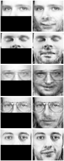
Results of the MADE model conditioned on the first half of the images.
Last words
Once you see it, it looks so simple. That’s probably the case with most good ideas. I really like the simplicity of this architecture. We were able to create a generative model (learning $P(x)$, just by applying masks to an autoencoder. The research made for the MADE paper, formed the basis for even more generative models as PixelRNN/ CNN (creating images pixel for pixel) and even the very cool wavenet (speech synthesis). I must mention that inference with this model architecture is super slow. This is due to the autoregressive properties of the model. During training, this isn’t an issue as all data points in the future $x_{t+n}$ are already known. At inference time, we need to predict them one by one, without any parallelization. This slow inference time is the reason why next post won’t be about Autoregressive flows. Instead it will be about Inverse Autoregressive flows and we will use the the autoregressive we have discussed today. But first, weekend!
References
[1] Brendan Fortuner (2018, Aug 11) Machine Learning Glossary Retrieved from https://github.com/bfortuner/ml-cheatsheet
[2] Germain, Gregor & Larochelle (2015, Feb 12) MADE: Masked Autoencoder for Distribution Estimation. Retrieved from https://arxiv.org/abs/1502.03509
[3] NPTEL-NOC IITM (2019, Apr 19) Deep Learning Part - II (CS7015): Lec 21.2 Masked Autoencoder Density Estimator (MADE). Retrieved from https://youtu.be/lNW8T0W-xeE
[4] Hinton et al. (2012, Jul 3) Improving neural networks by preventing co-adaptation of feature detectors. Retrieved from https://arxiv.org/abs/1207.0580
[5] Karpathy, A (2018, Apr 22) pytorch-made. Retrieved from https://github.com/karpathy/pytorch-made