
Last posts we’ve investigated Bayesian inference through variational inference (post 1/post 2). In Bayesian inference, we often define models with some unknown model parameters $Z$, or latent stochastic variables $Z$. Given this model and some observed data points $D = \{ D_1, D_2, \dots, D_n \} $, we are interested in the true posterior distribution $P(Z|D)$. This posterior is often intractable and the general idea was to forgo the quest of obtaining the true posterior, but to accept that we are bounded to some easily parameterizable approximate posteriors $^*Q(z)$, which we called variational distributions.
Variational inference has got some very cool advantages compared to MCMC, such as scalability and modulare usage in combination with deep learning, but it has also got some disadvantages. As we don’t know the optimal ELBO (the loss we optimize in VI), we don’t know if we are ‘close’ to the true posterior, and this constraint of ’easy’ parameterizable distributions used as family for $Q(z)$ often leads us to use distributions that aren’t expressive enough for the true non-gaussian real world.
This post we’ll explore a technique called normalizing flows. With NF are able to transform an ’easy’ paramaterizable base distribution in a more complex approximation for the posterior distribution. This is done by passing the base distribution through a series of transformations (the flow part). One of the definitions of a probability distribution is that the integral sums to one $\int_{-\infty}^{\infty} P(x) dx = 1$. A transformation can break this requirement, therefore we need to normalize $P(x)$ after the transformation.
1. Change of variables
First we are going to look at some basics. We are going to start of with basis distribution $\mathcal{N}(\mu=1, \sigma=0.1)$. In the code snippet below (the whole jupyter notebook is on github) we define this distribution in python and we apply a nummerical integral with np.trapz to validate the integral summing to 1.
x = np.linspace(0.01, 2, num=100)
base = stats.norm(1, 0.1)
print(np.trapz(base.pdf(x), x))
>>> 1.
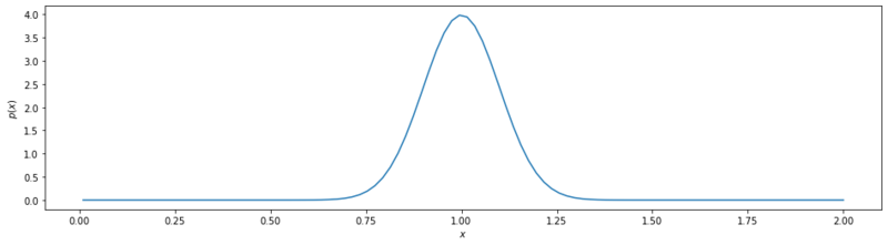
Basis Gaussian.
1.1 Transformation
Now we are going to apply a transformation $f(x) = x^2$.
def f(x):
    return x**2

y = f(x)
transformed = f(base.pdf(x))
print(np.trapz(transformed, y))
>>> 5.641895835477563
Transformed base wo/ normalization.
By applying this transformation we’ve blown up the probability space $\int_{-\infty}^{\infty} P(y) dy \gg 1$. We need a to modify this tranformation such that the integral over the entire domain evaluates to 1. Let’s define this a little bit more formally. We want to transform $P(x)$ to another distribution $P(y)$ with $f: \mathbb{R}^n \mapsto \mathbb{R}^n $. Because naively applying any possible $f$, would expand or shrink the probability mass of the distributions we need to constraint $f$ such that:
To hold this constraint we need to multiply $P(x)$ with the derivative of $x$ w.r.t. $y$, $\frac{dx}{dy}$. Therefore we need to express $x$ in $y$, which can only be done if the transformation $f$ is invertible.
Now we can rewrite eq. $ \eqref{normtransf}$ in terms of eq. $\eqref{invert}$:
1.1.1 1D verification
Let’s verify this in Python. Besides $f(x) = x^2$, we need $f^{-1}(y) = \sqrt(y)$ and $f’^{-1}(y) = \frac{1}{2 \sqrt(y)}$.
def f_i(y):
    return y**0.5

def f_i_prime(y):
    return 0.5*y**-0.5

assert np.allclose(f_i(f(x)),  x)

y = f(x)
px = base.pdf(x)
transformed = px * f_i_prime(f_i(y))
print(np.trapz(transformed, y))
>>> 0.9987379589284238
Transformed base w/ normalization.
Save some small deviation due to nummerical discretization, the transformation sums to 1! We can also observe this in the plot we’ve made. Because of the transformation, the resulting probability distribution has become wider, wich (in case of a Gaussian distribution) must result in a less high probability peak, if the total probability mass is preserved.
1.2 Conditions
The function $f(x) = x^2$ we’ve used in the example above was strictly increasing (over the domain $\mathbb{R}_{>0}$). This leads to a derivative $\frac{df}{dx}$ that is always positive. If we would have chosen a strictly decreasing function $g$, $\frac{dg}{dx}$ would always be negative. In that case eq. $\eqref{normtransf}$ would be defined as $P(y) = - P(x) \frac{dy}{dx}$. We could however, by taking the absolute value of the derivative, easily come up with an equation that holds true for both cases:
The intuition of taking the modulus can be seen as ensuring yourself that if the local rate of change for $x$ and $y$ are equal and increasing, the total amount of probability is preserved.
$$\begin{equation} x + dx = y + dy > 0 \end{equation}$$

Ensuring increasing probability.
1.3 Multiple dimensions
In multiple dimensions, the derivative $\frac{dx}{dy}$ is expressed in the determinant of the Jacobian matrix. Let $f: \mathbb{R}^n \mapsto \mathbb{R}^m$. The jacobian is a 2D matrix that stores the first order partial derivatives of all the outputs $\{f_1, f_2, \dots, f_m \}$ (the height of the matrix) w.r.t. all the inputs $\{x_1, x_2, \dots, x_n \}$ (the width of the matrix).
The dimensions of the probability distribution may not change due to the transformation, thus $f: \mathbb{R}^m \mapsto \mathbb{R}^m$ leading to a square jacobian matrix $m \times m$. From a square matrix, we can determine the determinant. The determinant of a matrix $A$ tells us how much an N-dimensional volume is scaled by applying the transformation $A$. For N-dimensions, eq. $\eqref{Py}$ is written with the determinant jacobian matrix.
1.3.1 2D verification
Again, let’s verify this in Python. Below we’ll define a two-dimensional random variable $X$ as a Gaussian distribution. We will also verify the integral condition, again by using np.trapz, but now over 2 dimensions.
# field of all possible events X
x1 = np.linspace(1, 5, num=50)
x2 = np.linspace(1, 5, num=50)
x1_s, x2_s = np.meshgrid(x1 ,x2)
x_field = np.concatenate([x1_s[..., None], x2_s[..., None]], axis=-1)

# distribution
base = stats.multivariate_normal(mean=[3, 3], cov=0.5)

# plot distribution
plt.contourf(x1_s, x2_s, base.pdf(x_field))

# Check if P(x) sums to one.
print(np.trapz(np.trapz(base.pdf(x_field), x_field[:, 0, 1], axis=0), x_field[0, :, 0]))
0.9905751293230018
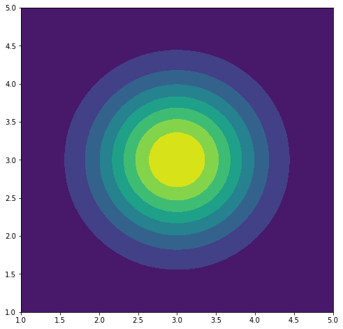
Probability distribution of $X$.
Next we have 2D function $f(x_1, x_2) = (e^{\frac{x_1}{3}}, x_2^2)$ and it’s inverse $f^{-1}(y_1, y_2) = (3\log y_1, \sqrt(y_2))$. We could also define the derivative of the inverse function, but as I am lazy we will use pytorch for automatic gradients.
def f(x1, x2):
    return torch.exp(x1 / 3), x2**2

def f_i(y1, y2):
    return 3 * torch.log(y1), y2**0.5

x_field = torch.tensor(x_field)
# Transform x events to y events
y_field = np.concatenate(f(x_field[..., 0, None], x_field[..., 1, None]), axis=-1)
Next we will need to define the jacobian matrix. For the purpose of this post, we’ll use a rather slow implementation, favoring readability.
def create_det_jac(y_field):
    # create for every y1, y2 combination the determinant of the jacobian f_i(y1, y2)
    det_jac = np.zeros((y_field.shape[0], y_field.shape[1]))
    for i in range(y_field.shape[0]):
        for j in range(y_field.shape[1]):
            y_field = torch.tensor(y_field)
            y_field.requires_grad_(True);
            fiy = torch.cat(f_i(y_field[..., 0, None], y_field[..., 1, None]), dim=-1)
            fiy[i, j].sum().backward()

            # Ouputs of the partial derivatives are independent.
	    # I.e. f1 is dependent of y1 and not y2
            # and vice versa f2 is dependent of y2 and not y1
            # therefore the multiplication w/ 0
            row1 = y_field.grad[i, j].data.numpy() * np.array([1., 0.])
            row2 = y_field.grad[i, j].data.numpy() * np.array([0., 1.])

            det = np.linalg.det(np.array([row1, row2]))
            det_jac[i, j] = det
    return det_jac
Now we’ve got all we need to do a distribution transformation and normalize the outcome.
px = base.pdf(x_field)
transformed = px * np.abs(create_det_jac(y_field))

# show contour plot
plt.contourf(y_field[..., 0], y_field[..., 1], transformed)

print(np.trapz(np.trapz(transformed, y_field[:, 0, 1], axis=0), y_field[0, :, 0]))
>>> 0.9907110850291531
Probability distribution of $Y$.
As we can see, we’ve transformed the base distribution while meeting the requirement of $\int P(y)dy=1$ by normalizing. Now we can continue applying these transformations in variational inference.
2. Normalizing flows
2.1 Single flow
Consider a latent variable model, with a latent variable $Z$ we’d like to infer. We choose a variational distribution $Q(z)$ over the latent variables $Z$. If we now have a invertible transformation $f: \mathbb{R}^m \mapsto \mathbb{R}^m$. A transformation of the latent variable $z’ = f(z)$, would have distribution $Q(z’)$.
Note: by applying the inverse function theorem, $J_{f^-1}(q) = [J_f(p)]^{-1}$, we can rewrite the determinant in terms of the function $f$ instead of it’s inverse $f^{-1}$, and $z$ instead of $z’$, and the multiplication becomes a division because of the inverse matrix $A^{-1}$ ($\log(A^{-1} = -\log A$). The inverse matrix notation should not be confused with inverse function notation.
2.2 K-flows
Because the flows have to be invertible, they are not likely to be very complex. Luckily, many simple transformations lead to more complex transformations. We like to obtain a complex random variable $Z_k$, by passing a simple random variable $Z_0$ through multiple flows, a flow composition.
\begin{eqnarray} z_k = f_k \circ \dots \circ f_2 \circ f1(z_0) \end{eqnarray}
Eq. $\eqref{Qz1}$ for $k$ flows becomes:
2.3 Variational Free Energy
The variation free energy is the optimization function we need to minimize. For more information about the derivation of this function read this post. For clarity, we are going the rearange the variational free energy as defined in my vi post, to the form used by Rezende & Mohammed in [1].
Now we have the same definition as [1], we can update $F(x)$ with $\log Q(z_K)$ (eq. $\eqref{qzk}$). Eq. $\eqref{vfepaper}$ then becomes:
2.4 Planar flows
$\mathcal{F}(x)$ is now general for any kind of normalizing flow, let’s investigate one such flow called planar flow. The planar flow transformation is defined as:
\begin{equation} f(z) = z + u h(w^Tz + b) \end{equation}
Here $\{ z \in \mathbb{R}^D, u \in \mathbb{R}^D, b\in \mathbb{R} \}$ are parameters we need to find by optimization. The function $h(\cdot)$ needs to be a smooth non linear function (the writers recommend using $\tanh(\cdot)$). Determining a determinant jacobian can be a very expensive operation, for invertible neural networks they are at least $\mathcal{O}(D^3)$. Besides the invertibility constraint, cheaply computed log determinant jacobians should also be taken into consideration, if you wanted to design your own flows. With planar flows it has been. The complexity is reduced to $\mathcal{O}(D)$, by using the matrix determinant lemma $\det(I + uv^T) = (1 + v^Tu)$.
That’s all we need! We can plug this determinant jacobian right in eq. $\eqref{vfeflow}$ and wrap it up. There are however some conditions that need to be met to guarantee invertibility. In appendix A of [1] they are explained.
3. Flow in practice
Okay, let’s see if we can bring what we’ve defined above in practice. In the snippet below we define a Planar class, the implementation of the flow that we’ve just discussed. Furthermore we normalize some of the parameters of the flow conform the appendix A in [1].
class Planar(nn.Module):
    def __init__(self, size=1, init_sigma=0.01):
        super().__init__()
        self.u = nn.Parameter(torch.randn(1, size).normal_(0, init_sigma))
        self.w = nn.Parameter(torch.randn(1, size).normal_(0, init_sigma))
        self.b = nn.Parameter(torch.zeros(1))

    @property
    def normalized_u(self):
        """
        Needed for invertibility condition.

        See Appendix A.1
        Rezende et al. Variational Inference with Normalizing Flows
        https://arxiv.org/pdf/1505.05770.pdf
        """

        # softplus
        def m(x):
            return -1 + torch.log(1 + torch.exp(x))

        wtu = torch.matmul(self.w, self.u.t())
        w_div_w2 = self.w / torch.norm(self.w)
        return self.u + (m(wtu) - wtu) * w_div_w2

    def psi(self, z):
        """
        ψ(z) =h′(w^tz+b)w

        See eq(11)
        Rezende et al. Variational Inference with Normalizing Flows
        https://arxiv.org/pdf/1505.05770.pdf
        """
        return self.h_prime(z @ self.w.t() + self.b) @ self.w

    def h(self, x):
        return torch.tanh(x)

    def h_prime(self, z):
        return 1 - torch.tanh(z) ** 2

    def forward(self, z):
        if isinstance(z, tuple):
            z, accumulating_ldj = z
        else:
            z, accumulating_ldj = z, 0
        psi = self.psi(z)

        u = self.normalized_u

        # determinant of jacobian
        det = (1 + psi @ u.t())

        # log |det Jac|
        ldj = torch.log(torch.abs(det) + 1e-6)

        wzb = z @ self.w.t() + self.b

        fz = z + (u * self.h(wzb))

        return fz, ldj + accumulating_ldj
3.1 Target distribution
Next we define a target distribution that is more complex than a standard Gaussian.
def target_density(z):
    z1, z2 = z[..., 0], z[..., 1]
    norm = (z1**2 + z2**2)**0.5
    exp1 = torch.exp(-0.2 * ((z1 - 2) / 0.8) ** 2)
    exp2 = torch.exp(-0.2 * ((z1 + 2) / 0.8) ** 2)
    u = 0.5 * ((norm - 4) / 0.4) ** 2 - torch.log(exp1 + exp2)
    return torch.exp(-u)
If we plot the density of function above we obtain the following target distribution.
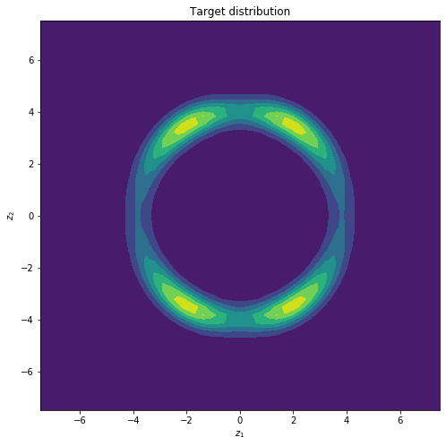
Target distribution we want to approximate.
3.2 Variational Free Energy
Eq. $\eqref{vfeflow}$ is defined below in the function det_loss. The joint probability $P(x, z_K)$ in $\eqref{vfeflow}$ is split in the likelihood (the target density case) and the prior $P(z_K)$ (which is note used as I use a uniform prior).
def det_loss(mu, log_var, z_0, z_k, ldj, beta):
    # Note that I assume uniform prior here.
    # So P(z) is constant and not modelled in this loss function
    batch_size = z_0.size(0)

    # Qz0
    log_qz0 = dist.Normal(mu, torch.exp(0.5 * log_var)).log_prob(z_0)
    # Qzk = Qz0 + sum(log det jac)
    log_qzk = log_qz0.sum() - ldj.sum()
    # P(x|z)
    nll = -torch.log(target_density(z_k) + 1e-7).sum() * beta
    return (log_qzk + nll) / batch_size
3.3 Final model
The single Planar layer is sequentially stacked in the Flow class. The instance of this class is the final model and will be optimized in order to approximate the target distribution.
class Flow(nn.Module):
    def __init__(self, dim=2, n_flows=10):
        super().__init__()
        self.flow = nn.Sequential(*[
            Planar(dim) for _ in range(n_flows)
        ])
        self.mu = nn.Parameter(torch.randn(dim, ).normal_(0, 0.01))
        self.log_var = nn.Parameter(torch.randn(dim, ).normal_(1, 0.01))

    def forward(self, shape):
        std = torch.exp(0.5 * self.log_var)
        eps = torch.randn(shape)  # unit gaussian
        z0 = self.mu + eps * std

        zk, ldj = self.flow(z0)
        return z0, zk, ldj, self.mu, self.log_var
3.4 Training and results
Last we need is the train loop. This is just a function where we pass a model instance and apply some gradient updates.
def train_flow(flow, shape, epochs=1000):
    optim = torch.optim.Adam(flow.parameters(), lr=1e-2)

    for i in range(epochs):
        z0, zk, ldj, mu, log_var = flow(shape=shape)
        loss = det_loss(mu=mu,
                        log_var=log_var,
                        z_0=z0,
                        z_k=zk,
                        ldj=ldj,
                        beta=1)
        loss.backward()
        optim.step()
        optim.zero_grad()
The figure below shows the final results. As we can see, the planar flow layer isn’t quite flexible enough to approximate the target in one or two layers. We eventually seem to need ~16 layers to come full cirlce.
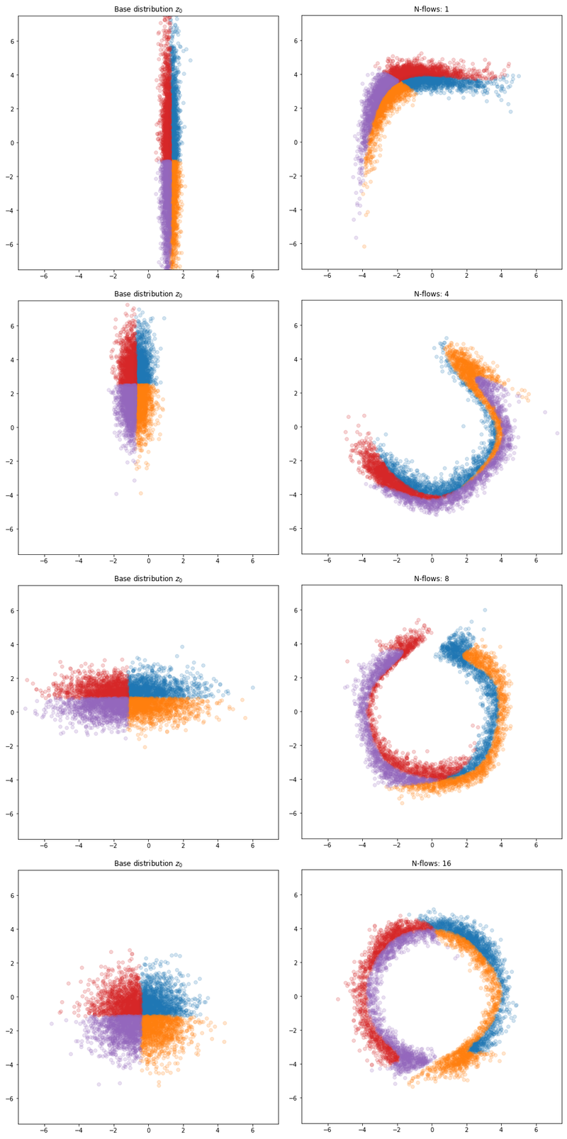
Results with different number of planar flows.
Discussion
Upgrading the variational distribution with normalizing flows addresses a core setback of variational inference, that of simplifying the posterior distribution too much. However, we remain limited to invertible functions. As we see in the example with the planar flows, we need quite some layers in order to obtain the flexible distribution. In higher dimensions this problem increases, and planar flows are often thought to be too simplistic. Luckily there are more complex transformations. Maybe I’ll discuss them in another post.
References
[1] Rezende & Mohammed (2016, Jun 14) Variational Inference with Normalizing Flows. Retrieved from https://arxiv.org/pdf/1505.05770.pdf
[2] Rippel & Adams (2013, Feb 20) High-Dimensional Probability Estimation with Deep Density Models. Retrieved from https://arxiv.org/pdf/1302.5125.pdf
[3] van den Berg, R (2018, Aug 11) Sylvester normalizing flows for variational inference Retrieved from https://github.com/riannevdberg/sylvester-flows