
Bayesian modeling! Every introduction on that topic starts with a quick conclusion that finding the posterior distribution often is computationally intractable. Last post I looked at Expectation Maximization, which is a solution of this computational intractability for a set of models. However, for most models, it isn’t. This post I will take a formal definition of the problem (As I’ve skipped that in the Expectation Maximization post) and we’ll look at two solutions that help us tackle this problem; Markov Chain Monte Carlo and Variational Inference.
0. Bayes’ formula
Bayes’ formula is a way to reverse conditional probability. It is quite elegant and if we apply it on machine learning we often find Bayes’ formula in the following form:
$$ P(\theta|D) = \frac{P(D|\theta) P(\theta)}{P(D)}$$
Let’s say we’ve defined a model architecture and we want to find the most likely parameters $\theta$ (a large vector, containing all the parameters from the model) for that model, given a set of observed data points $D$. This is what we are interested in, and this is called the posterior: $P(\theta|D)$. We often have some prior belief about the value of our parameters. For example, in a neural network, we often initialize our weights following a Gaussian distribution with a zero mean and unit variance. We believe that the true weights should be somewhere in that distribution. We call that our prior; $p(\theta)$. Given all values of $\theta$, we can compute the probability of observing our data. This is called the likelihood $P(D|\theta)$. And finally, we have a term, often called the evidence, $P(D)$. This is where the problems begin, as this is the marginal likelihood where all the parameters are marginalized.
$$ P(D) = \int_{\theta} P(D| \theta) P(\theta) \text{d} \theta $$
This integral is the problem. At even moderately high dimensions of $\theta$ the amount numerical operations explode.
1. Simple example
Let’s base this post on a comprehensible example (courtesy of our Xomnia statistics training). We will do a full Bayesian analysis in Python by computing the posterior. Later we will assume that we cannot. Therefore we will approximate the posterior (we’ve computed) with MCMC and Variational Inference.
Assume that we have observed two data points; $D=\{195, 182\}$. Both are observed lengths in cm of men in a basketball competition.
import numpy as np
import matplotlib.pyplot as plt
from scipy import stats

lengths = np.array([195, 182])
1.1 Likelihood function
I assume that the distribution of the true weights (the posterior) follow a Gaussian distribution. A Gaussian is parameterized with a mean $\mu$ and variance $\sigma^2$. For a reasonable domain of these parameters $\theta = \{ \mu , \sigma \}$ we can compute the likelihood $P(D|\theta) = P(D| \mu, \sigma)$.
computation domain
# lets create a grid of our two parameters
mu = np.linspace(150, 250)
sigma = np.linspace(0, 15)[::-1]

mm, ss = np.meshgrid(mu, sigma)  # just broadcasted parameters
likelihood
likelihood = stats.norm(mm, ss).pdf(lengths[0]) * stats.norm(mm, ss).pdf(lengths[1])
aspect = mm.max() / ss.max() / 3
extent = [mm.min(), mm.max(), ss.min(), ss.max()]
# extent = left right bottom top

plt.imshow(likelihood, cmap='Reds', aspect=aspect, extent=extent)
plt.xlabel(r'$\mu$')
plt.ylabel(r'$\sigma$')
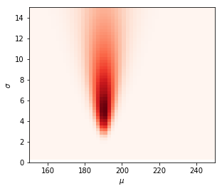
Likelihood function results
As we can see, the likelihood function represents the most likely parameters. If we would infer the most likely parameters $\theta$ based on only the likelihood we would choose the darkest red spots in the plot. By eyeballing it, I would say that $\mu=190$ and $\sigma=5$.
1.2 Prior distribution
Besides the likelihood, Bayes’ rule allows us to also include our prior belief in estimating the parameters. I actually believe most basketball players are longer. I believe the means follow a Gaussian distribution:
$$ \mu \sim \mathcal{N}(200, 15^2)$$
And that the variance $\sigma^2$ comes from a Cauchy distribution:
$$ \sigma \sim \mathcal{Cauchy}(0, 10^2)$$
prior = stats.norm(200, 15).pdf(mm) * stats.cauchy(0, 10).pdf(ss)

plt.imshow(prior, cmap='Greens', aspect=aspect, extent=extent)
plt.xlabel(r'$\mu$')
plt.ylabel(r'$\sigma$')
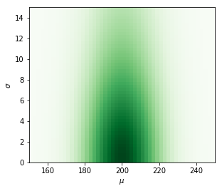
Prior distribution.
1.3 Posterior distribution
As we now have a simple model, not more than two dimensions, and a reasonable idea in which domain we need to search, we can compute the posterior directly by applying Bayes’ rule.
unnormalized_posterior = prior * likelihood
posterior = unnormalized_posterior / np.nan_to_num(unnormalized_posterior).sum()
plt.imshow(posterior, cmap='Blues', aspect=aspect, extent=extent)
plt.xlabel(r'$\mu$')
plt.ylabel(r'$\sigma$')
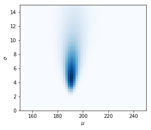
Posterior distribution.
This was easy. Because we weren’t cursed by high dimensions. Increase the dimensions, or define a more complex model, and the calculation of $P(D)$ becomes intractable.
2. Markov Chain Monte Carlo (MCMC)
One tool to tackle this intractability problem is Markov Chain Monte Carlo or MCMC.
In the plot showing the posterior distribution we first normalized the unnormalized_posterior by adding this line;
posterior = unnormalized_posterior / np.nan_to_num(unnormalized_posterior).sum(). The only thing this did was ensuring that the integral over the posterior equals 1; $\int_{\theta} P(\theta|D) \text{d}\theta =1$. This is necessary if we want the posterior distribution to be a probability distribution as one of the properties of a probability distribution is that the sum of all probability is 1!
However, if we would plot our unnormalized posterior, we would see exactly the same plot.
plt.imshow(unnormalized_posterior, cmap='Blues', aspect=aspect, extent=extent)
plt.xlabel(r'$\mu$')
plt.ylabel(r'$\sigma$')
Unnormalized posterior distribution.
This is because the normalization does not change the relative probabilities of $\theta_i$. This insight is very important and means that the posterior is proportional to the joint probability of $P(\theta, D)$, i.e. prior times likelihood.
$$ P(\theta|D) = \propto P(D|\theta)P(\theta)$$
So we don’t have to compute the evidence $P(D)$ to infer which parameters are more likely! However, making a grid over all of $\theta$ with a reasonable interval (which is what we did in our example), is still very expensive.
It turns out that we don’t need to compute $P(D|\theta)P(\theta)$ for every possible $\theta_i$ (or any reasonable grid approximation), but that we can sample $\theta_i$ proportional to the probability mass. This is done by exploring $\theta$ space by taking a random walk and computing the joint probability $P(\theta, D)$ and saving the parameter sample of $\theta_i$ according to the following probability:
$$ P(\text{acceptance}) = \text{min}(1, \frac{P(D|\theta^*)P(\theta^*)}{P(D|\theta)P(\theta)}$$
Where $\theta=$ current state, $\theta^*=$ proposal state.
The proposals that were accepted are samples from the actual posterior distribution. This is of course very powerful, as we are able to directly sample from, and therefore approximate, the real posterior!
Now we can see the relation with the name of the algorithm.
- Markov Chain: A chain of events, where every new event depends only on the current state; Acceptance probability.
- Monte Carlo: Doing something at random; Random walk through $\theta$ space.
If you want to get a solid intuition to why the acceptance ratio leads to samples from the posterior, take a look at Statistical Rethinking, Chapter 8: Markov chain Monte Carlo Estimation by Richard McElreath.
2.1 PyMC3
A Python package that does MCMC is PyMC3. Below we will show that MCMC works by modeling our example in PyMC3.
with pm.Model():
    # priors
    mu = pm.Normal('mu', mu=200, sd=15)
    sigma = pm.HalfCauchy('sigma', 10)

    # likelihood
    observed = pm.Normal('observed', mu=mu, sd=sigma, observed=lengths).
    # sample
    trace = pm.sample(draws=10000, chains=1)
fig, axes = plt.subplots(2, sharex=True, sharey=True, figsize = (16, 6))
axes[0].imshow(posterior, cmap='Blues', extent=extent, aspect=1)
axes[0].set_ylabel('$\sigma$')
axes[1].scatter(trace['mu'], trace['sigma'], alpha=0.01)
axes[1].set_ylabel('$\sigma$')
axes[0].set_title('True posterior')
axes[1].set_title('Sampled $\\theta$')
plt.xlabel('$\mu$')
plt.xlim(150, mm.max())
plt.ylim(0, ss.max())
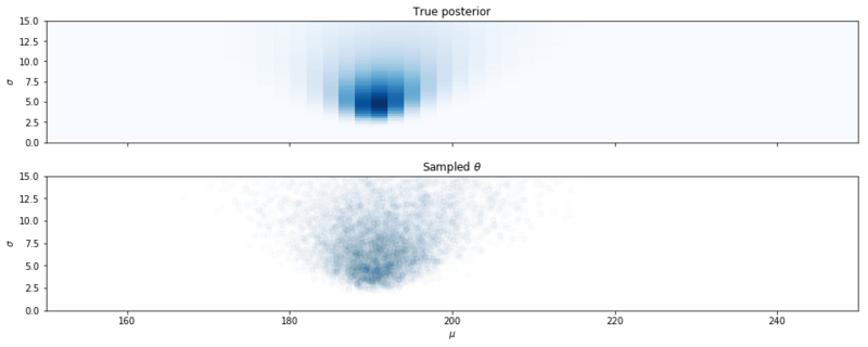
Samples from the posterior distribution with MCMC.
Above we clearly see that the samples obtained with MCMC are from the posterior distribution. Given enough samples, we can be assured that we have sampled the true probability density. The algorithm can be quite slow, but for a large number of models, it is fast enough.
3. Variational Inference
If we go into the realm of deep learning with large datasets and potentially millions of parameters
$\theta$, sampling with MCMC is often too slow. For this kind of problems, we rely on a technique called Variational Inference. Instead of computing the distribution, or approximating the real posterior by sampling from it, we choose an approximated posterior distribution and try to make it resemble the real posterior as close as possible.
The drawback of this method is that our approximation of the posterior can be really off.
The benefit is that it is an optimization problem with flowing gradients, which in the current world of autograd isn’t a problem at all!
Before reading further, I would recommend reading my Expectation Maximization post. In that post explore the derivation of the ELBO (Evidence Lower BOund), which turns out to be very important for Variational Inference.
3.1 Approximate distribution
We don’t know the real posterior so we are going to choose a distribution $Q(\theta)$ from a family of distributions $Q^*$ that is easy to work with, and parameterized by $\theta$. $Q(\theta)$ should resemble the posterior as closely as possible for the family $Q^*$. This ‘closeness’ is going to be measured by the Kullback-Leibler divergence.
Below this goal is shown visually. From a set of easy to work with distributions, we choose the one with the minimal KL-divergence w.r.t. the actual posterior distribution.

Search an approximation $Q(\theta$) that is 'close' to the posterior.
3.2 Kullback-Leibler to ELBO
Now your head should be filled with question marks!
How can we compute the KL-divergence $D_{\text{KL}}(Q(\theta) \: || \: P(\theta|D))$ when we don’t know the posterior?! It turns out that is the reason we’ve chosen KL-divergence (and not a real metric such as Wasserstein distance between $Q(\theta)$ and $P(\theta|D)$). With KL-divergence we don’t have to know the posterior! Below we’ll see why:
$$ D_{\text{KL}}(Q(\theta) \: || \: P(\theta|D)) = \int_{\theta} Q(\theta) \log \frac{Q(\theta)}{P(\theta|D)}\text{d}\theta $$
If we rewrite the posterior as $\frac{P(\theta, D)}{P(D)}$, we obtain:
$$ D_\text{KL} = \int_{\theta} Q(\theta) \log \frac{Q(\theta)P(D)}{P(\theta, D)}\text{d}\theta $$
Then we apply the logarithm rule of multiplication $\log (A \cdot B) = \log A + \log B$:
As $P(D)$ is not parameterized by $\theta$ and $\int_{\theta} Q(\theta) \text{d} \theta = 1$ we can write:
$$ D_\text{KL} = \int_{\theta} Q(\theta) \log \frac{Q(\theta)}{P(\theta, D)}\text{d}\theta + \log P(D) $$
By yet applying another log rule; $\log A = -\log \frac{1}{A}$ we obtain:
$$ D_\text{KL} = \log P(D) -\int_{\theta} Q(\theta) \log \frac{P(\theta, D)}{Q(\theta)}\text{d}\theta $$
And now we can see that the second term on the rhs is actually the ELBO, which can be written in expectation (over $\theta$) form.
$$ D_\text{KL} = \log P(D) - E_{\theta \sim Q}[\log \frac{P(\theta, D)}{Q(\theta)} ] $$
Now comes the key insight; The KL-divergence range is always positive. That means that in order to minimize KL-divergence we need to maximize the ELBO and we don’t need to know the value of $P(D)$.
In the Expectation Maximization post we see another derivation of the ELBO (the lower bound on the evidence $P(D)$. In that post we derived it using Jensen’s Inequality.
The ELBO is something we can compute as it only contains the approximation distribution $Q(\theta)$ (which we determine), and the joint probability $P(\theta, D)$, i.e. the prior times the likelihood!
In the derivation of Variational Autoencoders, the ELBO is often written in two terms; a reconstruction error and a KL-term on the variational distribution $Q_\theta$ and the prior $P(\theta)$
First we rewrite the joint probability $P(\theta, D)$ into conditional probability $P(D|\theta)P(\theta)$.
$$ \text{ELBO} = E_{\theta \sim Q}[\log \frac{P(D|\theta)P(\theta)}{Q(\theta)} ] $$
Then we expand the equation and thereby isolating the reconstruction error $\log P(D|\theta)$, i.e. the log likelihood.
$$ \text{ELBO} = E_{\theta \sim Q}[\log P(D|\theta)] + E_{\theta \sim Q}[\log \frac{P(\theta)}{Q(\theta)}]$$
If we rewrite the $E_{\theta \sim Q}[\log \frac{P(\theta)}{Q(\theta)}]$ in the integral form $\int_{\theta} Q(\theta)\log\frac{P(\theta)}{Q(\theta)}d\theta$, we can observe that this is the KL-divergence between the prior $P(\theta)$ and the variational distribution $Q(\theta)$. Resulting in an ELBO defined by the reconstruction error and $-D_{KL}(Q(\theta)||P(\theta)).$
$$ \text{ELBO} = E_{\theta \sim Q}[\log P(D|\theta)] - D_{KL}(Q(\theta)||P(\theta))$$
3.3 Mean Field Approximation
Once we’ve defined a model, we need to define a distribution $Q(\theta)$ that approximates the posterior. One approach is called the Mean Field Approximation. Note that the joint probability is defined by:
$$ P(A,B) = P(A|B)P(B) $$
If $A$ is independent of $B$, the above simplifies to:
$$ P(A,B) = P(A) P(B) $$
Let’s redefine what we are doing here. The first step is approximating the posterior (a conditional probability) with a variational distribution (a joint probability).
$$ P(\theta|D) \approx Q(\theta) $$
Then we define the variational distribution as a product of independent partitions of $\theta$ (the partitions can span multiple dimensions, but can also be one dimensional).
$$ Q_\text{mfa}(\theta) = \prod_{i=1}^N Q_i(\theta_i) $$
Where the partitioned distribution is often chosen to be from an exponential family. By defining a mean field approximation we end up with an ’easy to work with’ distribution, which is parameterized the same way as the posterior.
The only thing that lasts now is finding the variational parameters of $Q_\text{mfa}(\theta)$ through optimization.
3.4 Variational Inference in Pyro
There are several ways to solve this optimization problem. One solution is stochastic gradient descent. This requires computing gradients, which we don’t want to do by hand. Therefore we are going to use [Pyro](Deep Universal Probabilistic Programming). This is a probabilistic programming language based on Pytorch. First, we are going to define the generative model just as we did in PyMC3.
import pyro
import pyro.optim
import pyro.distributions as dist
from pyro.infer import SVI, Trace_ELBO
import torch
import torch.distributions.constraints as constraints


def model():
    # priors
    mu = pyro.sample('mu', dist.Normal(loc=torch.tensor(200.),
                                       scale=torch.tensor(15.)))
    sigma = pyro.sample('sigma', dist.HalfCauchy(scale=torch.tensor(10.)))

    # likelihood
    with pyro.plate('plate', size=2):
        pyro.sample(f'obs', dist.Normal(loc=mu, scale=sigma),
                    obs=torch.tensor([195., 185.]))
Then we are going to define the variational distribution $Q(\theta)$, in pyro, this is called the guide.
def guide():
    # variational parameters
    var_mu = pyro.param('var_mu', torch.tensor(180.))
    var_mu_sig = pyro.param('var_mu_sig', torch.tensor(5.),
                             constraint=constraints.positive)
    var_sig = pyro.param('var_sig', torch.tensor(5.))

    # factorized distribution
    pyro.sample('mu', dist.Normal(loc=var_mu, scale=var_mu_sig))
    pyro.sample('sigma', dist.Chi2(var_sig))
It is important that the guide samples from the same named random variables (defined by pyro.sample). This counts for all random variables except the likelihood (has the obs keyword argument). In the guide, we define how the posterior approximation is distributed. In our case we assume mu to be normally distributed, and that sigma is drawn from a Chi-squared distribution. Those approximated posterior distributions are parameterized by variational parameters. Not the parameters $\theta$ we try to infer! Pyro will adjust those variational parameters using Stochastic Variational Inference (SVI) guided by the ELBO loss.
Below we optimize our guide, conditioned on our model. We use clipped gradients as the data isn’t scaled.
pyro.clear_param_store()
pyro.enable_validation(True)

svi = SVI(model, guide,
          optim=pyro.optim.ClippedAdam({"lr":0.01}),
          loss=Trace_ELBO())

# do gradient steps
c = 0
for step in range(5000):
    c += 1
    loss = svi.step()
    if step % 100 == 0:
        print("[iteration {:>4}] loss: {:.4f}".format(c, loss))
After we have done inference, we can initialize our approximated distributions and sample from them.
sigma = dist.Chi2(pyro.param('var_sig')).sample((10000,)).numpy()
mu = dist.Normal(pyro.param('var_mu'), pyro.param('var_mu_sig')).sample((10000,)).numpy()
fig, axes = plt.subplots(2, sharex=True, sharey=True, figsize = (16, 6))
axes[0].imshow(posterior, cmap='Blues', extent=extent, aspect=1)
axes[0].set_ylabel('$\sigma$')
axes[1].scatter(mu, sigma, alpha=0.1)
axes[1].set_ylabel('$\sigma$')
axes[0].set_title('True posterior $P(\\theta|D)$')
axes[1].set_title('Approximated posterior $Q(\\theta)$')
plt.xlabel('$\mu$')
plt.xlim(150, mm.max())
plt.ylim(0, ss.max())
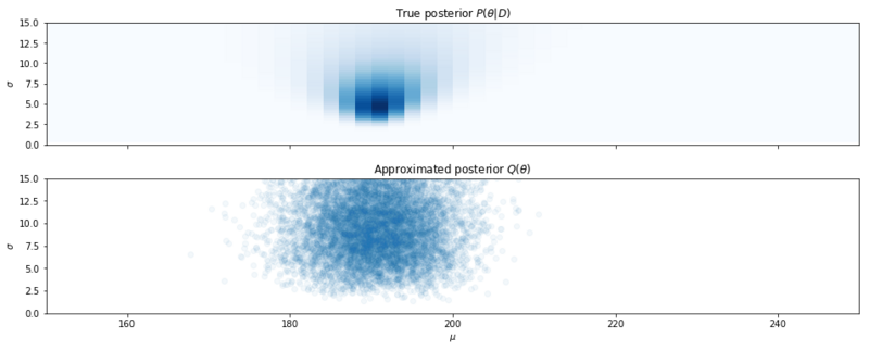
Samples from the Mean Field Approximation.
Above we see the result. As we can see, the variational distribution isn’t a perfect approximation and is of course greatly influenced by how we choose our variational distributions. But it is a technique that is usable with models with large numbers of parameters. And in neural networks, where we have such numeric violence, I guess a Gaussian approximation is pretty OK, no matter what the data looks like.
TL;DR
$$ Q(\theta) \approx P(\theta|D) $$ The code of this post can be found on github.