I wanted to learn something about variational inference, a technique used to approximate the posterior distribution in Bayesian modeling. However, during my research, I bounced on quite some mathematics that led me to another optimization technique called Expectation Maximization. I believe the theory behind this algorithm is a stepping stone to the mathematics behind variational inference. So we tackle the problems one problem at a time!
The first part of this post will focus on Gaussian Mixture Models, as expectation maximization is the standard optimization algorithm for these models. The second part of the post, we will focus on a broader view on expectation maximization, and we will get the mathematical intuition of what we are optimizing.
Gaussian Mixture Model
The schoolbook example of Expectation Maximization starts with a Gaussian Mixture model. Below we will go through the definition of a GMM in 1D, but note that this will generalize to ND. Gaussian Mixtures help with the following clustering problem. Assume a generative process where $X$ is an observed random variable.
$$ z_i \sim Multionomial(\phi) $$ $$ x_i|z_i \sim N(\mu_k, \sigma_k^2) $$
$x_i$ is sampled from two different Gaussians. $z_i$ is an unobserved variable that determines from which Gaussian is sampled. Note that in this 1D case, the Multinomial distribution is the Bernoulli distribution. The parameter $\phi_j$ gives $p(z_i = j)$. We could generate this data in Python as follows:
import matplotlib.pyplot as plt
import numpy as np
from scipy import stats

np.random.seed(654)
# Draw samples from two Gaussian w.p. z_i ~ Bernoulli(phi)
generative_m = np.array([stats.norm(2, 1), stats.norm(5, 1.8)])
z_i = stats.bernoulli(0.75).rvs(100)
x_i = np.array([g.rvs() for g in generative_m[z_i]])

# plot generated data and the latent distributions
x = np.linspace(-5, 12, 150)
plt.figure(figsize=(16, 6))
plt.plot(x, generative_m[0].pdf(x))
plt.plot(x, generative_m[1].pdf(x))
plt.plot(x, generative_m[0].pdf(x) + generative_m[1].pdf(x), lw=1, ls='-.', color='black')
plt.fill_betweenx(generative_m[0].pdf(x), x, alpha=0.1)
plt.fill_betweenx(generative_m[1].pdf(x), x, alpha=0.1)
plt.vlines(x_i, 0, 0.01, color=np.array(['C0', 'C1'])[z_i])
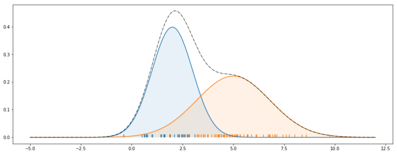
Generative process Gaussian Mixture Models.
The picture above clearly depicts the generative process of a Gaussian Mixture model. The dashed line shows $p(x_i; \theta)$. The blue Gaussian shows $p(x_i|z_i=1; \theta)$, and the orange Gaussian shows $p(x_i|z_i=2; \theta)$. Note that $\theta$ are the distribution parameters, $\mu$, $\sigma$ and $\phi$.
If $Z$ was an observed variable we would know that all data points would come from two Gaussians and for each single data point we could tell from which Gaussian it has originated.

$X$ and $Z$ are observed.
In such a case we could model the joint distribution $p(x_i, z_i) = p(x_i| z_i) p(z_i)$ (i.e. fit the Gaussians) by applying maximum likelihood estimation. However, in an unsupervised case $Z$ is latent and all we observe is $X$.

$X$ is observed
With observing only $X$, it has become a lot harder to determine $p(x_i, z_i)$, as we are not sure by which Gaussian $x_i$ is produced.
Expectation Maximization in GMM
The log-likelihood of the model is defined below, but as $Z$ is unobserved, the log-likelihood function has no closed form for the maximum likelihood.
$$\ell(\theta) = \sum_{i=1}^n \text{log} p(x_i; \theta)$$
$$\ell(\theta) = \sum_{i=1}^n \text{log} \sum_{k=1}^K p(x_i| z_k; \theta) p(z_k; \theta)$$
Because of this, we will use an optimization algorithm called Expectation Maximization, where we guess $Z$ and iteratively try to maximize the log-likelihood.
E-step
Given a set of initialized chosen (or updated) parameters we determine $w_{ij}$ for each data point.
$$ w_{ij} := p(z_i = j|x_i; \theta)$$
Asking the questions, what is the likelihood of data point $x_i$, being assigned to Gaussian $j$.
M-step
Now we are going to optimize the parameters by applying an algorithmic step, quite similar to K-means, but now we are weighing them with the likelihoods $w_{ij}$. In K-means, we have a hard cut off, and determine the new means from the data points assigned to the cluster from the previous iteration. Now we will use all the data points for determining the new mean, but we scale them.
$$ \phi_j := \frac{1}{n}\sum_{i=1}^n w_{ij} $$ $$ \mu_j := \frac{\sum_{i=1}^nw_{ij} x_i} {\sum_{i=1}^nw_{ij}} $$ $$ \sigma_j := \sqrt{\frac{\sum_{i=1}^nw_{ij}(x_i - \mu_j)^2} {\sum_{i=1}^nw_{ij}}} $$
If we iterate the E-M steps, we hope to converge to maximum likelihood. (The log-likelihood function, is multi-modal so we could get stuck in a local optimum)
Python example
Below we have implemented the algorithm in Python.
class EM:
    def __init__(self, k):
        self.k = k
        self.mu = None
        self.std = np.ones(k)
        self.w_ij = None
        self.phi = np.ones(k) / k

    def expectation_step(self, x):
        for z_i in range(self.k):
            self.w_ij[z_i] = stats.norm(self.mu[z_i], self.std[z_i]).pdf(x) * self.phi[z_i]
	# normalize zo that marginalizing z would lead to p = 1
	self.w_ij /= self.w_ij.sum(0)

    def maximization_step(self, x):
        self.phi = self.w_ij.mean(1)
        self.std = ((self.w_ij * (x - self.mu[:, None])**2).sum(1) / self.w_ij.sum(1))**0.5
        self.mu = (self.w_ij * x).sum(1) / self.w_ij.sum(1)

    def fit(self, x):
        self.mu = np.random.uniform(x.min(), x.max(), size=self.k)
        self.w_ij = np.zeros((self.k, x.shape[0]))

        last_mu = np.ones(self.k) * np.inf
        while ~np.all(np.isclose(self.mu, last_mu)):
            last_mu = self.mu
            self.expectation_step(x)
            self.maximization_step(x)

m = EM(2)
m.fit(x_i)
We can examine the final fit by reparameterizing the two Gaussians once the algorithm has converged.
fitted_m = [stats.norm(mu, std) for mu, std in zip(m.mu, m.std)]

plt.figure(figsize=(16, 6))
plt.vlines(x_i, 0, 0.01, color=np.array(['C0', 'C1'])[z_i])
plt.plot(x, fitted_m[0].pdf(x))
plt.plot(x, fitted_m[1].pdf(x))
plt.plot(x, generative_m[0].pdf(x), color='black', lw=1, ls='-.')
plt.plot(x, generative_m[1].pdf(x), color='black', lw=1, ls='-.')
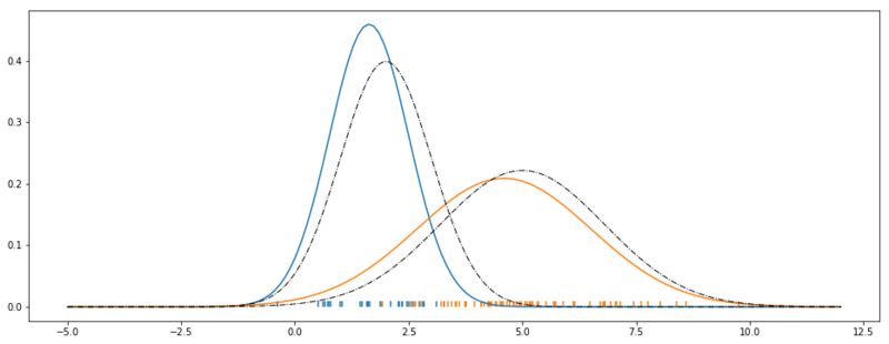
Optimized Gaussian Mixture Model.
As we can see. We have a reasonable fit. The black dashed lines show the original data generating Gaussians. The blue and the orange Gaussians are the result of our parameter search.
General Expectation Maximization
Above we’ve shown EM in relation to GMMs. However, EM can be applied in a more general sense to a wider range of algorithms. We noted earlier that we cannot optimize the log-likelihood directly because we haven’t observed $Z$. It turns out that we can find a lower bound to the log-likelihood function, which we can optimize.
In the figure below, we see the intuition behind optimizing a lower bound on the log-likelihood. A lower bound $g$ of $f$ exists if $g(x) \leq f(x)$ for all $x$ in its domain.
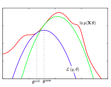
Iteratively maximizing a lower bound of $\ell(\theta)$.
Jensen’s inequality
How do we obtain a lower bound function of the log-likelihood? Jensen’s inequality theorem states that for every strictly concave function $f$ (i.e. $f^{\prime\prime} < 0$ for the whole domain range $x$) applied on a random variable $X$:
Jensen’s inequality: $$ E[f(X)] \leq f(E[X]) $$
This inequality will be an equality if and only if $X = E[X]$ with probability 1. In other words, if $X$ is a constant.
Jensen’s equality: $$ E[f(X)] = f(E[X]) \text{ iff } X = E[X]$$
Below we’ll get some intuition for the theorem. We define a range of $x := (0, 15)$, take $\log$ as our function $f(x)$ and compute the lhs and rhs of Jensens inequality. For plotting purposes, the theorem is applied on the full range $(0, 15)$, where we would normally apply it to samples from a probability distribution.
x = np.linspace(1, 15)

plt.figure(figsize=(16, 6))
plt.title('Log(x) is concave')
plt.plot(x, np.log(x))
plt.annotate(r'$f(x)$', (13, np.log(13) + 0.1))

plt.hlines(np.log(np.mean(x)), 0, np.mean(x), linestyles='-.', lw=1)
plt.annotate(r'$f(E[x])$', (0, np.log(np.mean(x)) + 0.1))

plt.hlines(np.mean(np.log(x)), 0, np.exp(np.mean(np.log(x))), linestyles='-.', lw=1)
plt.annotate(r'$E[f(x)])$', (0, np.mean(np.log(x)) - 0.15))
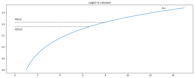
Jensen's inequality applied on $(0, 15)$.
Evidence Lower Bound ELBO
Now we are going to define a lower bound function on the evidence $p(x)$. This marginal likelihood over $Z$ is often intractable, as we need to integrate over all possible values of $z_i$ to compute it.
Recall that we try to optimize the evidence $p(X; \theta)$ under the current guess of the parameters $\theta$.
$$ \ell(\theta) = p(X; \theta) = \sum_{i=1}^n \log p(x_i; \theta)$$
As we assume a latent variable $Z$ which we haven’t observed, we can rewrite it including $z_i$ (which is marginalized out).
$$ \ell(\theta) = \sum_{i=1}^n\log\sum_{z_i}p(x_i, z_i; \theta)$$
Now we can multiply the equation above with an arbitrary distribution over $Z$, $\frac{Q(z)}{Q(z)}=1$.
$$ \ell(\theta) = \sum_{i=1}^n\log\sum_{z_i} Q(z_i) \frac{p(x_i, z_i; \theta)} {Q(z_i)}$$
Now note that expectation of a random variable $X$ is defined as $E[X] = \sum_{i=1}^n p(x_i)x_i$. Which means we can rewrite the log-likelihood as
$$ \ell(\theta) = \sum_{i=1}^n\log E_{z \sim Q}[\frac{p(x_i, z; \theta)} {Q(z)}]$$
As the $\log$ function is a concave function, we can apply Jensen’s inequality to the right-hand side of the equation. Note that we put the $\log$ inside the expectation.
$$ \sum_{i=1}^n\log E_{z \sim Q}[\frac{p(x_i, z; \theta)} {Q(z)}] \geq \underbrace{\sum_{i=1}^n E_{z \sim Q}[ \log \frac{p(x_i, z; \theta)} {Q(z)}]}_{\text{lower bound of }\ell(\theta) = p(x; \theta)}$$
Now we continue with this lower bound of $p(X; \theta)$ and unpack the expectation in the summation form.
$$ \ell(\theta) \geq \sum_{i=1}^n\log\sum_{z_i} Q(z_i) \log \frac{p(x_i, z_i; \theta)} {Q(z_i)}$$
The equation above holds true for every distribution we choose for $Q(z)$, but ideally, we choose a distribution that leads to a lower bound that is close to the log-likelihood function. It turns out we can choose a distribution that will make the lower bound equal to $p(X; \theta)$. This is due to the fact that Jensen’s inequality holds to equality if and only if $X = E[X]$, i.e. $X$ is constant. Where $X$, in this case, is part inside the $\log$ function; $ \frac{p(x_i, z_i; \theta)} {Q(z_i)}$.
Therefore we must choose a distribution of $Q(z)$ that leads to:
$$ \frac{p(x_i, z_i; \theta)}{Q(z_i)} = 1$$
Which means that
$$ p(x_i, z_i; \theta) \propto Q(z_i) $$
And because $Q(z)$ is a probability distribution, it must integrate to one; $\sum_{z_i}Q(z_i) = 1$. So ideally we want to take the joint distribution $p(x_i, z_i ; \theta)$ and transform it so that it is proportional to itself, but also sums to 1 over all values of $z_i$. It turns out we can find that by normalizing the joint distribution.
$$ \sum_{z_i} \frac{p(x_i, z_i; \theta)}{\sum_{z_i} p(x_i, z_i; \theta)} = 1 $$
We can rewrite the equation inside the summation to a conditional probability.
$$ Q(z_i) = \frac{p(x_i, z_i; \theta)}{\sum_{z_i} p(x_i, z_i; \theta)} $$
$$ Q(z_i) = \frac{p(x_i, z_i; \theta)}{p(x_i; \theta)} $$
$$ Q(z_i) = p(z_i | x_i; \theta)$$
And that leaves us with the final form of lower bound on the log-likelihood (ELBO).
$$ \log p(x; \theta) \geq \text{ELBO}(x; Q, \theta) $$
Relation to Expectation Maximization
In the section above, we’ve found a lower bound on the log-likelihood for the current values of $\theta$ and $Q(z)$. And our goal is to optimize $\theta$ so that we maximize the log-likelihood $\log p(x; \theta)$. Because we cannot optimize this function directly we try to optimize its lower bound $\sum_{i=1}^n\log\sum_{z_i} Q(z_i) \log ( \frac{p(x_i, z_i; \theta)} {Q(z_i)}) $.
This lower bound was equal to the log-likelihood if we choose $Q(z) = p(z|x; \theta)$. On the current parameters $\theta_t$ and $Q(z)$, we optimize to $\theta_{t+1}$. However, once we do the optimization step, Jensen’s equality doesn’t hold anymore, as $Q(z)$ is still parameterized on the previous parameter step $\theta_t$. For these reasons we optimize in two steps;
- The Expectation step: Under current parameters $\theta_t$, find $Q(z) = p(z| x; \theta_t)$
- The Maximization step: With $Q(z; \theta_t)$, optimize the lower bound of the log-likelihood: $\underset{\theta}{\arg\max}\text{ELBO}(x; Q, \theta)$ so that we obtain $\theta_{t+1}$.
Which is exactly what we did in our earlier Gaussian Mixture example. We set $w_{ij} := p(z_i = j|x_i; \theta, \phi)$, and then we used $w_{ij}$ to find $\theta_{t+1}$, and thus increasing the log-likelihood.
Further readings
In an earlier post, we also took a look at Gaussian Mixture Models. In the example in this post, k was a hyperparameter of the algorithm. In the post about Dirichlet Mixtures, we don’t specify k, but we use Dirichlet processes to inferr k, which means that we do non parametric clustering!