Clustering data with Dirichlet Mixtures in Edward and Pymc3

Last post I’ve described the Affinity Propagation algorithm. The reason why I wrote about this algorithm was because I was interested in clustering data points without specifying k, i.e. the number of clusters present in the data.

This post continues with the same fascination, however now we take a generative approach. In other words, we are going to examine which models could have generated the observed data. Through bayesian inference we hope to find the hidden (latent) distributions that most likely generated the data points. When there is more than one latent distribution we can speak of a mixture of distributions. If we assume that the latent distribrutions are Gaussians than we call this model a Gaussian Mixture model.

First we are going to define a bayesian model in Edward to determine a multivariate gaussian mixture model where we predifine k. Just as in k-means clustering we will have a hyperparameter k that will dictate the amount of clusters. In the second part of the post we will reduce the dimensionality of our problem to one dimension and look at a model that is completely nonparametric and will determine k for us.

Dirichlet Distribution

Before we start with the generative model, we take a look at the Dirichlet distribution. This is a distribution of distributions and can be a little bit hard to get your head around. If we sample from a Dirichlet we’ll retrieve a vector of probabilities that sum to 1. These discrete probabilites can be seen as seperate events. A Dirichlet distribution can be compared to a bag of badly produced dice, where each dice has a totally different probability of throwing 6. Each time you sample a die from the bag you sample another probabilty of throwing 6. However you still need to sample from the die. Actually throwing the die will lead to sampling the event.

The Dirichlet distribution is defined by:

where

If we want to create a Dirichlet distribution in three dimensions we need to initialize it with $\alpha = [\alpha_1, \alpha_2, \alpha_3]$. The expected value of $\theta$ becomes:

import numpy as np
from scipy import stats
import matplotlib.pyplot as plt
from mpl_toolkits.mplot3d import Axes3D

for alpha in [[1, 3, 4], [1, 1, 1], [10, 0.2, 0.2], [0.1, 0.1, 0.1]]:
    theta = stats.dirichlet(alpha).rvs(500)

    fig = plt.figure(figsize=(8, 8), dpi=150)
    ax = plt.gca(projection='3d')
    plt.title(r'$\alpha$ = {}'.format(alpha))
    ax.scatter(theta[:, 0], theta[:, 1], theta[:, 2])
    ax.view_init(azim=30)
    ax.set_xlabel(r'$\theta_1$')
    ax.set_ylabel(r'$\theta_2$')
    ax.set_zlabel(r'$\theta_3$')
    plt.show()

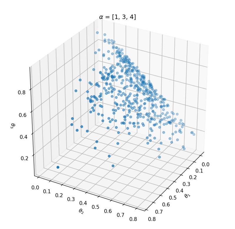
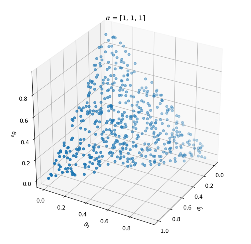
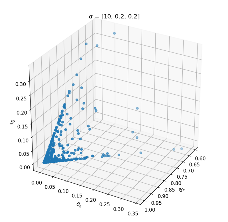
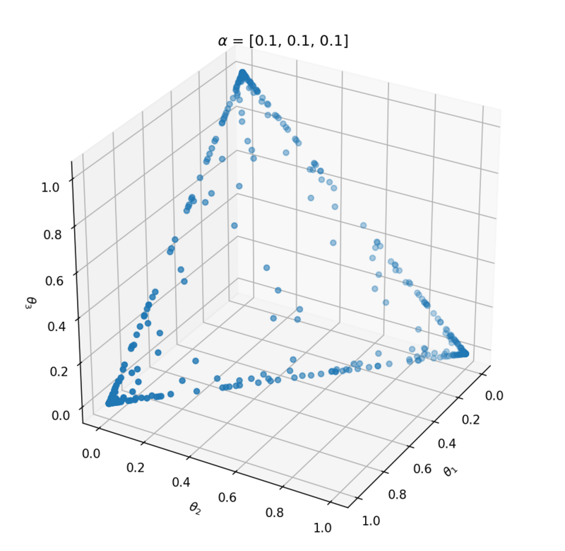
Above the underlying distribution of $Dir(\alpha)$ is shown by sampling from it. Note that $\alpha = [10, 0.2, 0.2]$ leads to high probability of $P(\alpha_1)$ close to 1 and that $\alpha = [1, 1, 1]$ can be seen as uniform Dirichlet distribution, i.e. that there is an equal probability for all distributions that suffices $\sum_{i=1}^{k}{\theta_i} = 1$.

Clustering with generative models

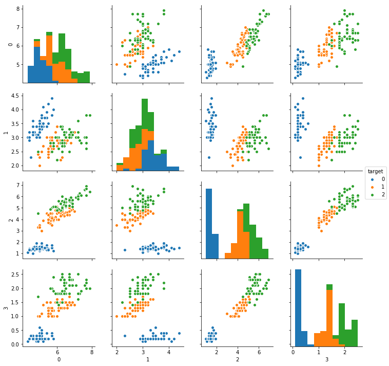
Now, we have had a nice intermezzo of Dirichlet distributions, we’re going to apply this distribution in a Gaussian Mixture model. We will try to cluster the Iris dataset. This is a dataset containing 4 columns of data gathered from 3 different types of flowers.

import pandas as pd
from sklearn.datasets import load_iris
import seaborn as sns
from scipy import stats
import tensorflow as tf
import edward as ed

df = pd.DataFrame(load_iris()['data'])
y = df.values
# Standardize the data
y = (y - y.mean(axis=0)) / y.std(axis=0)

# A 2D pairplot between variables
df['target'] = load_iris()['target']
sns.pairplot(df, hue='target', vars=[0, 1, 2, 3])

Gaussian Mixture

A Gaussian Mixture model is the Mother Of All Gaussians. For column 0 in our dataframe it is the cumulative of the histograms of the data labels.

plt.figure(figsize=(12, 6))
b = 8
a = 4

plt.title('MOAS')
plt.xlabel(r'$X$')
plt.ylabel('bin count')
plt.annotate('Cummulative distribution', (6.8, 17), (7, 20), arrowprops=dict(facecolor='black', shrink=0.05))
plt.hist(df[0], color=sns.color_palette()[3], rwidth=a)
plt.hist(df[0][df['target'] == 2], color=sns.color_palette()[2], rwidth=a)
plt.hist(df[0][df['target'] == 1], color=sns.color_palette()[1], rwidth=a)
plt.hist(df[0][df['target'] == 0], color=sns.color_palette()[0], rwidth=a)

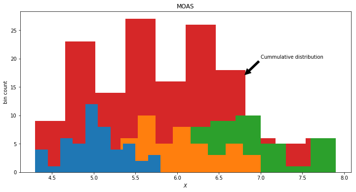
Of we obtain a dataset without labels. What we would observe from the world is the single red distribution. However we know now that the data actually is produced by the 3 latent distributions, namely three different kind of flowers. The red observed distribution is a mixture of the hidden distributions. We could model this by choosing a mixture of 3 Gaussian distributions

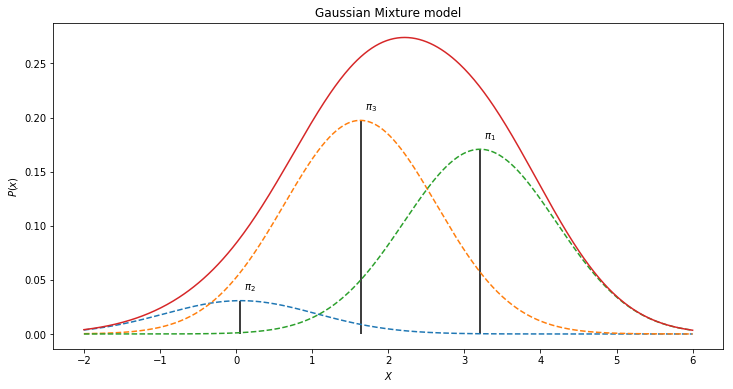
However the integral of a Gaussian distribution is equal to 1 (as a probability function should be). If we combine various Gaussians we need to weigh them so the integral will meet the conditon of being equal to 1.

We could of course scale the mixture of Gaussian by weights summing to 1. Here comes the Dirichlet distribution in place. Every sample from a Dirichlet sums to one and could be used as weights to scale down the mixture of Gaussian distributions.

The final generative model can thus be defined by:

where $\pi$ are the weights drawn from $Dir(\alpha)$. One such mixture model for the histogram above for instance could look like:

np.random.seed(13)
x = np.linspace(-2, 6, 500)
pi = stats.dirichlet([1, 1, 1]).rvs()[0]
mu = stats.norm(1, 1).rvs(3)

y = stats.norm(mu, np.ones(3)).pdf(x[:, None])
plt.figure(figsize=(12, 6))
plt.title('Gaussian Mixture model')
plt.ylabel(r'$P(x)$')
plt.xlabel(r'$X$')

plt.plot(x, y[:, 1] * pi[1], ls='--')
plt.plot(x, y[:, 2] * pi[2], ls='--')
plt.plot(x, y[:, 0] * pi[0], ls='--')

for i in range(3):
    xi = x[np.argmax(y[:, i])]
    yi = (y[:, i] * pi[i]).max()
    plt.vlines(xi, 0, yi)
    plt.text(xi + 0.05, yi + 0.01, r'$\pi_{}$'.format(i + 1))
plt.plot(x, (y * pi).sum(1))

Generative model in Edward

The model defined in eq. (2.1) is conditional on $\pi$, $\mu$ and $\sigma$. We don’t know the values of these variables, but as we are going to use bayesian inference we can set a prior probability on them. The priors we choose:

We can define this generative model in Edward. First we define the priors and finally we combine them in a mixture of Multivariate Normal distributions.

k = 3  # number of clusters

d = df.shape[1]
n = df.shape[0]

pi = ed.models.Dirichlet(tf.ones(k))
mu = ed.models.Normal(tf.zeros(d), tf.ones(d), sample_shape=k)  # shape (3, 4) 3 gaussians, 4 variates
sigmasq = ed.models.InverseGamma(tf.ones(d), tf.ones(d), sample_shape=k)
x = ed.models.ParamMixture(pi, {'loc': mu, 'scale_diag': tf.sqrt(sigmasq)},
                 ed.models.MultivariateNormalDiag,
                 sample_shape=n)
z = x.cat

Now this model is defined we can start inferring from the observed data. To be able to do Gibbs sampling in Edward we need to define Empricial distributions for our priors.

t = 500  # number of samples

qpi = ed.models.Empirical(tf.get_variable('qpi', shape=[t, k], initializer=tf.constant_initializer(1 / k)))
qmu = ed.models.Empirical(tf.get_variable('qmu', shape=[t, k, d], initializer=tf.zeros_initializer()))
qsigmasq = ed.models.Empirical(tf.get_variable('qsigmasq', shape=[t, k, d], initializer=tf.ones_initializer()))
qz = ed.models.Empirical(tf.get_variable('qz', shape=[t, n], initializer=tf.zeros_initializer(), dtype=tf.int32)) 

And hit the magic infer button (this one actually belongs to Pymc3)!

inference = ed.Gibbs({pi: qpi, mu: qmu, sigmasq: qsigmasq, z: qz}, 
                    data={x: y})
inference.run()

Out:

500/500 [100%] ██████████████████████████████ Elapsed: 2s | Acceptance Rate: 1.000

Conditioned on our priors, Edward has now inferred the most likely posterior distribution given the data. The cool thing is that we can now sample from this posterior distribution and analize:

• The cluster assignment of the data points.
• The uncertainty of our inferred variables.
• Generate new data similar to our original dataset.

Uncertainty

Let’s sample from the posterior.

mu_s = qmu.sample(500).eval()
sigmasq_s = qsigmasq.sample(500).eval()
pi_s = qpi.sample(500).eval()

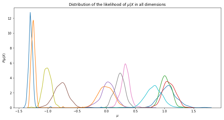
We can for instance get information about the uncertainty of our result by looking the distributions of our variables. By plotting this, we see that a value for $\mu$ is probably close to -1.3 (blue line) and that the model is pretty confident about this result as the width of the distribution is very small.

plt.figure(figsize=(12, 6))
plt.title(r'Distribution of the likelihood of $\mu | X$ in all dimensions')
plt.ylabel(r'$P(\mu|X)$')
plt.xlabel(r'$\mu$')
for i in range(3):
    for j in range(4):
        sns.distplot(mu_s[:, i, j], hist=False)

Cluster assignment

Clustering each datapoint is done by rebuilding our model from eq (2.1) with the inferred variables sampled from the posterior distribution and assign each datapoint to the Gaussian with the highest probability.

np.vstack([pi_s.mean(0)[i] * \
           stats.multivariate_normal(mu_s.mean(0)[i], np.sqrt(sigmasq_s.mean(0))[i]).pdf(y) \
           for i in range(3)]).argmax(axis=0)

Out:

array([2, 2, 2, 2, 2, 2, 2, 2, 2, 2, 2, 2, 2, 2, 2, 2, 2, 2, 2, 2, 2, 2,
       2, 2, 2, 2, 2, 2, 2, 2, 2, 2, 2, 2, 2, 2, 2, 2, 2, 2, 2, 2, 2, 2,
       2, 2, 2, 2, 2, 2, 0, 1, 0, 1, 1, 1, 0, 1, 1, 1, 1, 1, 1, 1, 1, 1,
       1, 1, 1, 1, 1, 1, 1, 1, 1, 1, 1, 0, 1, 1, 1, 1, 1, 1, 1, 1, 0, 1,
       1, 1, 1, 1, 1, 1, 1, 1, 1, 1, 1, 1, 0, 1, 0, 0, 0, 0, 1, 0, 0, 0,
       0, 0, 0, 1, 0, 0, 0, 0, 0, 1, 0, 1, 0, 1, 0, 0, 1, 1, 0, 0, 0, 0,
       0, 1, 1, 0, 0, 0, 1, 0, 0, 0, 1, 0, 0, 0, 1, 0, 0, 1])

By reversing the order we can look at the accuracy of our unsupervised learning model.

np.vstack([pi_s.mean(0)[i] * \
           stats.multivariate_normal(mu_s.mean(0)[i], np.sqrt(sigmasq_s.mean(0))[i]).pdf(y) \
          for i in range(3)])[::-1].argmax(axis=0).sum() / df.shape[0]

Out:

0.94

We have a accuracy of 94%. Which isn’t bad considered the fact that we do unsupervised learning here.

There is one thing however that still bothers me. We’ve put prior knowledge in this model, namely the number of clusters! We’ve instanciated our prior Dirichlet distribution with $\alpha = \vec{1}$. Hereby dictating the number of clusters we can weigh to sum op to 1. Wouldn’t it be neat, if we could define a model that is able to choose its number of clusters as it would see fit?

Dirichlet Process

The Dirichlet Process is just as the Dirichlet distribution also a distribution of discrete distributions. And this one could help us with a model that is able to define k for us.

If we sample from a Dirichlet Process, we’ll get a distribution of infinite discrete probabilities $\theta$.

The function of the Dirichlet Process is described by:

where

• $H_0$ is an original distribution by our choosing.
• $\pi_i$ are weights that sum to 1.
• $\delta$ is the Dirac delta function.
• $\theta$ are samples drawn from $H_0$.

$\pi$ are weights summing to one and can be defined by a metaphor called the stick breaking process, where we first sample infinite values $\pi’$ from a Beta distribution parameterized by $1$ and $\alpha$. We start with a whole stick and we will infinitly break of $1 - \pi’_i$ from the stick. The first iteration from the whole stick, the other iterations from the remaining part.

where

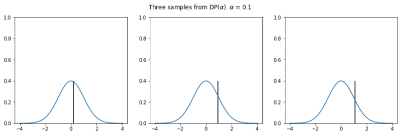
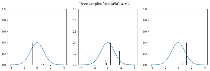
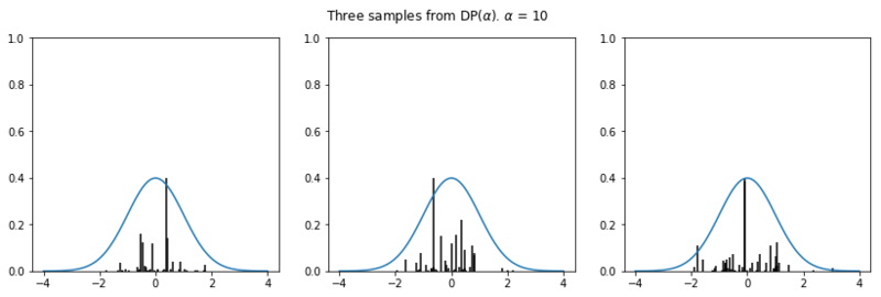
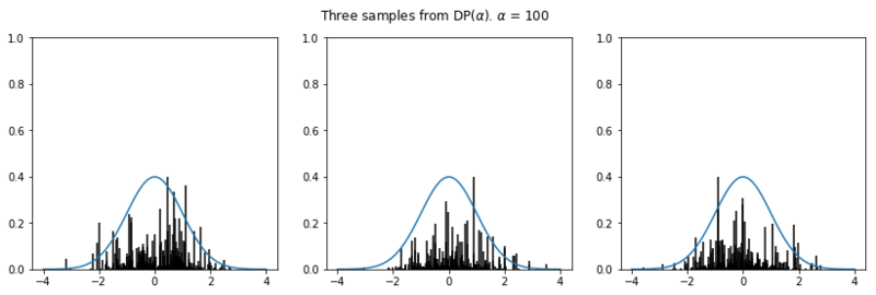
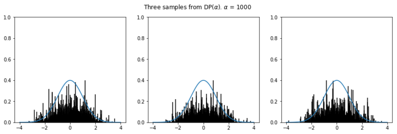
Ok, that was the formal definition. Let’s look at what it actually means to sample from a Dirichlet Process. Below we define a function where we simulate a Dirichlet Process. We simulate it because in real life it is impossible to sample an infinite amount of values. We truncate the amount of samples based on some heuristics, assuming that the sum of $\pi’$ will be approximating 1 with a negligible difference.

In the plots below we see the influence of $\alpha$ on the sampled distributions. As $H_0$ we choose the familiar Gaussian distribution. In every row we plot three distribution samples. Note that for higher values of $\alpha$, the sampled distribution $H$ will look closer to the original distribution $H_0$.

def dirichlet_process(h_0, alpha):
    """
    Truncated dirichlet process.
    :param h_0: (scipy distribution)
    :param alpha: (flt)
    :param n: (int) Truncate value.
    """
    n = max(int(5 * alpha + 2), 500)  # truncate the values. 
    pi = stats.beta(1, alpha).rvs(size=n)
    pi[1:] = pi[1:] * (1 - pi[:-1]).cumprod()  # stick breaking process
    theta = h_0(size=n)  # samples from original distribution
    return pi, theta
        
def plot_normal_dp_approximation(alpha, n=3):
    pi, theta = dirichlet_process(stats.norm.rvs, alpha)
    x = np.linspace(-4, 4, 100)
    
    plt.figure(figsize=(14, 4))
    plt.suptitle(r'Three samples from DP($\alpha$). $\alpha$ = {}'.format(alpha))
    plt.ylabel(r'$\pi$')
    plt.xlabel(r'$\theta$')
    pltcount = int('1' + str(n) + '0')
    
    for i in range(n):
        pltcount += 1
        plt.subplot(pltcount)
        pi, theta = dirichlet_process(stats.norm.rvs, alpha)
        pi = pi * (stats.norm.pdf(0) / pi.max())
        plt.vlines(theta, 0, pi, alpha=0.5)
        plt.ylim(0, 1)
        plt.plot(x, stats.norm.pdf(x))

np.random.seed(65)
for alpha in [.1, 1, 10, 100, 1000]:
    plot_normal_dp_approximation(alpha)

Nonparametric clustering

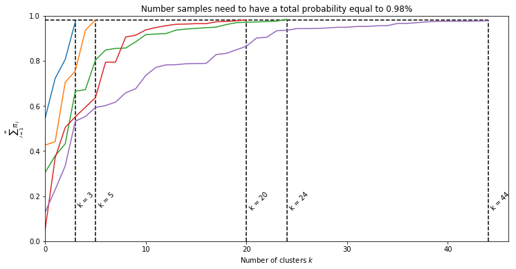
How can we use the Dirichlet Process in order to nonparametricly (thus without specifying k) define the number of clusters in the data? Well, we can actually use the same model as defined in eq (2.1). However instead of sampling from a Dirichlet distribution were we define the number of clusters with the parameter $\alpha$, we now sample from a Dirichlet Process and give a prior on the parameter $\alpha$. Parameter $\alpha$ influences how fast $\sum_{i=1}^{\infty}{\pi_i}$ approaches 1. If we accept only the clusters under a certain percentage the model can define by itself what value for $\alpha$ is most likely given the data. Below we can see how $\alpha$ influences the number of clusters when we accept a total probability of 98%.

np.random.seed(95)

acceptance_p = 0.98
plt.figure(figsize=(12, 6))
plt.title(f'Number samples need to have a total probability equal to {acceptance_p}%')
plt.ylabel('$\sum_{i=1}^{\infty}{\pi_i}$')
plt.xlabel('Number of clusters $k$')
def plot_summation(alpha):
    pi, _ = dirichlet_process(stats.norm.rvs, alpha)
    p_total = np.cumsum(pi)
    i = np.argmin(np.abs(p_total - acceptance_p))
    plt.plot(np.arange(pi[:i + 1].shape[0]), p_total[:i + 1])
    return i

k = 0
for alpha in [1, 2, 5, 7, 10]:
    k_i = plot_summation(alpha)
    k = max(k, k_i)
    plt.vlines(k_i, 0, acceptance_p, linestyles='--')
    plt.text(k_i + 0.2, 0.2, f'k = {k_i}', rotation=45)
    
plt.ylim(0, 1)
plt.xlim(0, k + 2)
plt.hlines(acceptance_p, 0, k, linestyles='--')

Dirichlet Process Mixtures in Pymc3

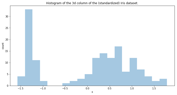
Now we are going to test a Dirichlet Process Mixture model in Pymc3. We are going to model the density of the data in one dimension. The data dimension we’ll be modelling is:

plt.figure(figsize=(12, 6))
plt.title('Histogram of the 3d column of the (standardized) Iris dataset.')
plt.xlabel('x')
plt.ylabel('count')
sns.distplot(y[:, 2], bins=20, kde=None)

The model we’ve described in eq (2.1) can be reshaped a little bit. By setting an extra prior on the $\alpha$ variable and a few other priors, we obtain the following model in Pymc3:

k = 35
m = pm.Model()
with m:
    alpha = pm.Gamma('alpha', 1, 1)
    beta = pm.Beta('beta', 1, alpha, shape=k)
    pi = pm.Deterministic('pi', stick_breaking(beta))

    tau = pm.Gamma('tau', 1, 1, shape=k) 
    lambda_ = pm.Uniform('lambda', 0, 1, shape=k)
    mu0 = pm.Uniform('mu0', -3, 3, shape=k)
    
    mu = pm.Normal('mu', mu=mu0, tau=1, shape=k)
    obs = pm.NormalMixture('obs', w=pi, mu=mu, tau=lambda_ * tau, observed=y[:, 2])

Above we’ve defined the priors and combined them in a NormalMixture. This Normal Mixture distribution is what we observe from the world. We pass the observed data in the observed keyword argument. Now we can sample from the posterior and infer the most likely distributions for our models variables.

with m: 
    trace = pm.sample(500, tune=500, init='advi', random_seed=35171)

Inferred k

We can examine the number of clusters by looking at the weight given to each Gaussian distribution.

plt.figure(figsize=(12, 6))
plt.title(r"Distribution of $\pi'$")
plt.bar(np.arange(k) + 1 - 0.5, trace['pi'].mean(axis=0), width=1., lw=0);
plt.xlim(0.5, k);
plt.xlabel('Component');
plt.ylabel('Posterior expected mixture weight');

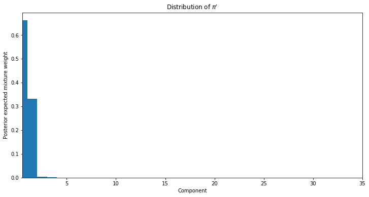
Above we see the weights $\pi’$ given to each Gaussian. Here it seems likely there are 2 clusters in our 1 dimensional dataset. As the weights given to any Gaussian with weigths < 0.3 are negligible and don’t give any significant mass to our Mixture of Gaussians.

Appreciate the fact that the number of clusters is defined by the value inferred for $\alpha$. Below we sample 6 times from the Dirichlet Process with the mean value inferred from $\alpha$. In these plots it is visible why our model gives most weights to 2 Gaussians and not to 15 Gaussians for instance.

plot_normal_dp_approximation(trace['alpha'].mean(), 6)

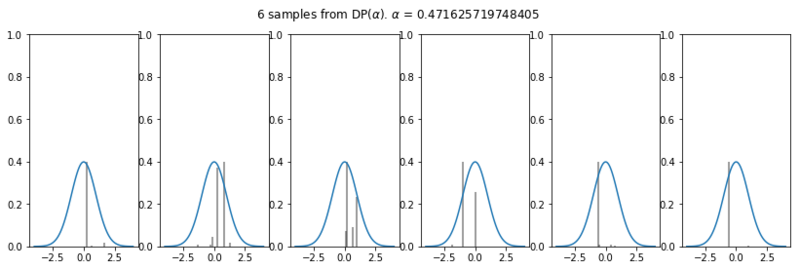
The number of weights drawn with a value > 0.01 varies between 1 and 4, hereby strongly influencing the number of clusters that are most likely according to the model.

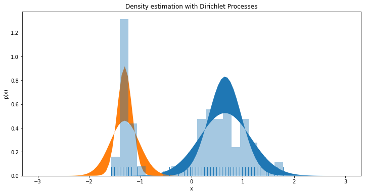
Finally lets look at how the models Gaussian Mixture compares to our dataset. We also plot the confidence interval between 0.05% - 0.95%. This is gives an indication of the uncertainty of the model. Below we’ve plotted the two most significant Gaussians and see that they describe the observed data very well. We only plot two, as the rest is negligible.

plt.figure(figsize=(12, 6))
plt.title('Density estimation with Dirichlet Processes')
plt.xlabel('x')
plt.ylabel('p(x)')
x = np.linspace(-3,  3, 100)
pi_mean = trace['pi'].mean(0)
mu_mean = trace['mu'].mean(0) 
mu0_mean = trace['mu0'].mean(0)
lambda_mean = trace['lambda'].mean(0)
tau_mean = trace['tau'].mean(0)
sd_mean = np.sqrt((1 / tau_mean * lambda_mean))
tau_sd = trace['mu'].std(0)
lambda_sd = trace['lambda'].std(0)
sd_sd = np.sqrt((1 / tau_sd * lambda_sd))

p = stats.norm.interval(0.05, trace['mu'].mean(0), trace['mu'].std(0))
psd = stats.norm.interval(0.05, sd_mean, sd_std)

a = 2
plt.fill_between(x, stats.norm.pdf(x, mu_mean[0], psd[0][0]) * pi_mean[0], stats.norm.pdf(x, mu_mean[0], psd[1][0]) * pi_mean[0])
plt.fill_between(x, stats.norm.pdf(x, mu_mean[1], psd[0][1]) * pi_mean[1], stats.norm.pdf(x, mu_mean[1], psd[1][1]) * pi_mean[1])
sns.distplot(y[:, 2], bins=20, kde=None, norm_hist=True, rug=True, )

Conclusion

We’ve seen two different generative models that utilize the Dirichlet distribution and the Dirichlet Process to cluster observed data. In the first model we defined the number of clusters as a hyperparameter. In the last model the number of clusters was defined nonparameterically by the model itself. The latter seems very powerful for data mining, however I did find it was harder to find the right hyperparameters for the priors than in the fixed cluster model and found that it to becomes much more complex if we want to do the same in multiple dimensions.

Read more!

• Affinity Propagation
• Gaussian Processes