
Christopher Fonnesbeck did a talk about Bayesian Non-parametric Models for Data Science using PyMC3 on PyCon 2018. In this talk, he glanced over Bayes’ modeling, the neat properties of Gaussian distributions and then quickly turned to the application of Gaussian Processes, a distribution over infinite functions. Wait, but what?! How does a Gaussian represent a function? I did not understand how, but the promise of what these Gaussian Processes representing a distribution over nonlinear and nonparametric functions really intrigued me and therefore turned into a new subject for a post. This post we’ll go, a bit slower than Christopher did, through what Gaussian Processes are.
In the first part of this post we’ll glance over some properties of multivariate Gaussian distributions, then we’ll examine how we can use these distributions to express our expected function values and then we’ll combine both to find a posterior distribution for Gaussian processes.
1. Introduction: The good old Gaussian distribution.
The star of every statistics 101 college, also shines in this post because of its handy properties. Let’s walk through some of those properties to get a feel for them.
A Gaussian is defined by two parameters, the mean $\mu$, and the standard deviation $\sigma$. $\mu$ expresses our expectation of $x$ and $\sigma$ our uncertainty of this expectation.
$$ x \sim \mathcal{N}(\mu, \sigma)$$
A multivariate Gaussian is parameterized by a generalization of $\mu$ and $\sigma$ to vector space. The expected value, i.e. the mean, is now represented by a vector $\vec{\mu}$. The uncertainty is parameterized by a covariance matrix $\Sigma$.
$$ x \sim \mathcal{N}(\mu, \Sigma) $$
The covariance matrix is actually a sort of lookup table, where every column and row represent a dimension, and the values are the correlation between the samples of that dimension. For this reason, it is symmetrical. As the correlation between dimension i and j is equal to the correlation between dimensions j and i.
$$\Sigma_{ij} = \Sigma_{ji}$$
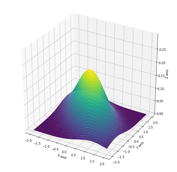
Below I have plotted the Gaussian distribution belonging $\mu = [0, 0]$, and $\Sigma = \begin{bmatrix} 1 && 0.6 \\ 0.6 && 1 \end{bmatrix}$.
Gaussians make baby Gaussians
Gaussian processes are based on Bayesian statistics, which requires you to compute the conditional and the marginal probability. Now with Gaussian distributions, both result in Gaussian distributions in lower dimensions.
Marginal probability
The marginal probability of a multivariate Gaussian is really easy. Officially it is defined by the integral over the dimension we want to marginalize over.
Given this jointly distribution:
The marginal distribution can be acquired by just reparameterizing the lower dimensional Gaussian distribution with $\mu_x$ and $\Sigma_x$, where normally we would need to do an integral over all possible values of $y$.
$$p(x) = \int{p(x, y)dy} = \mathcal{N}(\mu_x, \Sigma_x)$$
Below we see how integrating, (summing all the dots) leads to a lower dimensional distribution which is also Gaussian.
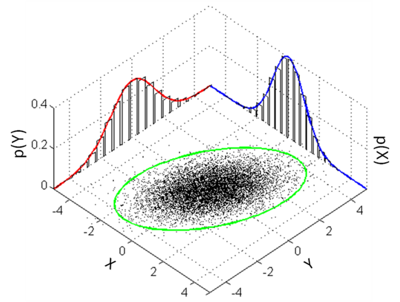
Marginal probability of a Gaussian distribution
Conditional probability
The conditional probability also leads to a lower dimensional Gaussian distribution.
Below is shown a plot of how the conditional distribution also leads to a Gaussian distribution (in red).
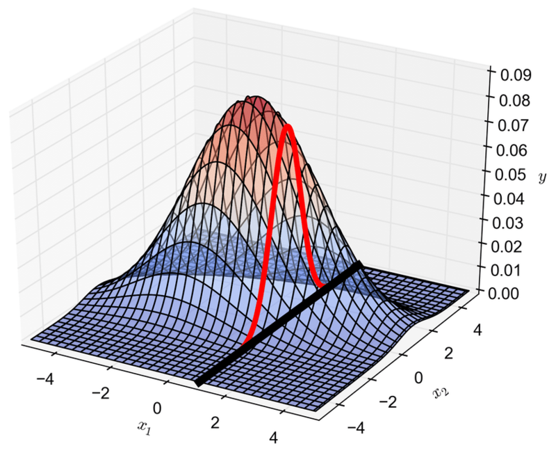
Conditional probability of a Gaussian distribution
2. Functions described as multivariate Gaussians
A function $f$, is something that maps a specific set (the domain) $X$ to another set (the codomain) $Y$.
$$ f(x) = y$$
The domain and the codomain can have an infinite number of values. But let’s imagine for now that the domain is finite and is defined by a set $X =$ {$ x_1, x_2, \ldots, x_n$}.
We could define a multivariate Gaussian for all possible values of $f(x)$ where $x \in X$.
Here the $\mu$ vector contains the expected values for $f(x)$. If we are certain about the result of a function, we would say that $f(x) \approx y$ and that the $\sigma$ values would all be close to zero. Each time we sample from this distribution we’ll get a function close to $f$. It is important to note that each finite value of x is another dimension in the multivariate Gaussian.
Let’s give an example in Python.
import numpy as np
import matplotlib.pyplot as plt
from scipy import stats


n = 50
x = np.linspace(0, 10, n)

# Define the gaussian with mu = sin(x) and negligible covariance matrix
norm = stats.multivariate_normal(mean=np.sin(x), cov=np.eye(n) * 1e-6)
plt.figure(figsize=(16, 6))

# Taking a sample from the distribution and plotting it.
plt.plot(x, norm.rvs())
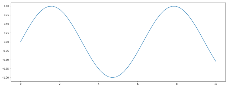
A function sampled from a Gaussian distribution.
We can also define a distribution of functions with $\vec{\mu} = 0$ and $\Sigma = I$ (the identity matrix). Now we do have some uncertainty because the diagonal of $\Sigma$ has a standard deviation of 1. A second thing to note is that all values of $f(x)$ are completely unrelated to each other, because the correlation between all dimensions is zero. In the example below, we draw 3 functions from this distribution.
# Define the gaussian with mu = 0 and a covariance matrix w/o any correlation,
# but w/ uncertainty
norm = stats.multivariate_normal(mean=np.zeros(n), cov=np.eye(n))
plt.figure(figsize=(16, 6))

# Taking 3 sample from the distribution and plotting it.
[plt.plot(x, norm.rvs()) for _ in range(3)]
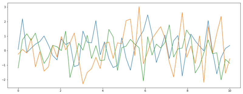
Three functions sampled from $\mathcal{N}(\vec{0}, I)$
3. Controlling the functions with kernels
As you can see we’ve sampled different functions from our multivariate Gaussian. In fact, we can sample an infinite amount of functions from this distribution. And if we would want a more fine grid of values, we could also reparameterize our Gaussian to include a new set of $X$.
However, these functions we sample now are pretty random and maybe don’t seem likely for some real-world processes. Let’s say we only want to sample functions that are smooth. Besides that smoothness looks very slick, it is also a reasonable assumption. Values that are close to each other in domain $X$, will also be mapped close to each other in the codomain $Y$. We could construct such functions by defining the covariance matrix $\Sigma$ in such a way that values close to each other have larger correlation than values with a larger distance between them.
Squared exponential kernel
A way to create this new covariance matrix is by using a squared exponential kernel. This kernel does nothing more than assigning high correlation values to $x$ values closely together.
$$k(x, x’) = exp(- \frac{(x-x’)^2}{2l^2})$$
If we now define a covariance matrix $\Sigma = k(x, x)$, we sample much smoother functions.
def kernel(m1, m2, l=1):
    return np.exp(- 1 / (2 * l**2) * (m1[:, None] - m2)**2)

n = 50
x = np.linspace(0, 10, n)
cov = kernel(x, x, 0.44)

norm = stats.multivariate_normal(mean=np.zeros(n), cov=cov)
plt.figure(figsize=(16, 6))
[plt.plot(x, norm.rvs()) for _ in range(3)]
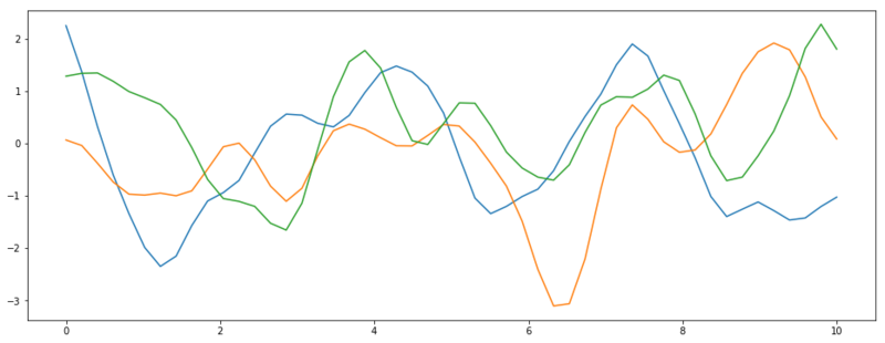
Three functions sampled from $\mathcal{N}(\vec{0}, k(x, x))$
4. Gaussian Processes
Ok, now we have enough information to get started with Gaussian processes. GPs are used to define a prior distribution of the functions that could explain our data. And conditional on the data we have observed we can find a posterior distribution of functions that fit the data. Let’s say we have some known function outputs $f$ and we want to infer new unknown data points $f_*$. With the kernel we’ve described above, we can define the joint distribution $p(f, f_*)$.
So now we have a joint distribution, which we can fairly easily assemble for any new $x_*$ we are interested in. Assuming standardized data, $\mu$ and $\mu_*$ can be initialized as $\vec{0}$. And all the covariance matrices $K$ can be computed for all the data points we’re interested in.
- $K = k(x, x)$
- $K_* = k(x, x_*)$
- $K_{**} = k(x_*, x_*)$
Because this distribution only forces the samples to be smooth functions, there should be infinitely many functions that fit $f$.
And now comes the most important part. Given a prior $f_{prior}$ Gaussian, wich we assume to be the marginal distribution, we can compute the conditional distribution $f_*|f$ (as we have observed $f$).. Which is something we can calculate because it is a Gaussian. However, to do so, we need to go through some very tedious mathematics. We will take this for granted and will only work with the end result. Gaussian processes for machine learning, presents the algebraic steps needed to compute this conditional probability. We’ll end up with the two parameters need for our new probability distribution $\mu_*$ and $\Sigma_*$, giving us the distribution over functions we are interested in.
$$f_* = \mathcal{N}(\mu_*, \Sigma_*)$$
A quick note, before we’ll dive into it. The resulting Gaussian probabilities are written in term of a unit Gaussian. Both of the next distributions are equal.
$$\mathcal{N}(\mu, \sigma) = \mu + \sigma \mathcal{N}(0, 1) $$
Setup
Next part of the post we’ll derive posterior distribution for a GP. Therefore we’ll need some test data. Let’s assume a true function $f = sin(x)$ from which we have observed 5 data points.
np.random.seed(512)
# True function
f = lambda x: np.sin(x)

# Known domain of true function f
x = np.random.uniform(0, 10, 5)

plt.figure(figsize=(16, 6))
plt.scatter(x, f(x))
plt.xlim(0, 10)
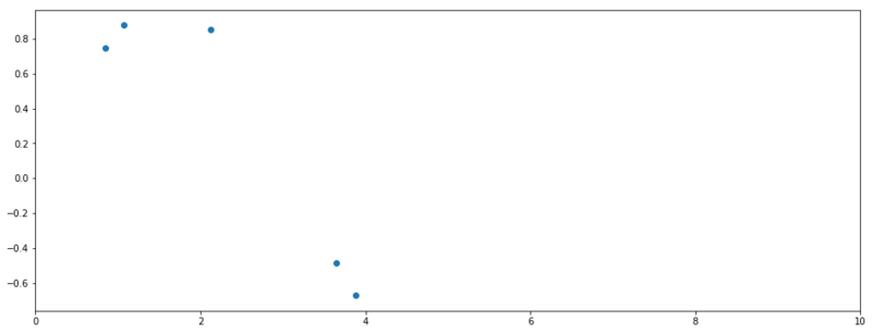
Observed values of $f$
Prior probability
We first set up the new domain $x_{*}$ (i.e. the features we want to predict) and apply the kernel $k_{**} = k(x_{*}, x_{*})$. This results in our new covariance matrix for our prior distribution. Instead of parameterizing our prior with this covariance matrix, we take the Cholesky decomposition $\text{cholesky}(k_{**})$, which in this context can be seen a square root operation for matrices and thus transforming the variance into the standard deviation. As we assume standardized data ($\mu = 0$), we can ignore $\mu_{*}$.
$$ p(f_{*}) = \text{cholesky}(k_{**}) \mathcal{N}(0, I) $$
n = 200
# Domain of f* we want to infer
x_s = np.linspace(0, 10, n)

# covariance matrix
K_ss = kernel(x_s, x_s, l=0.8)

# Is square root of matrix (standard deviation)
L_ss = np.linalg.cholesky(K_ss + 1e-6 * np.eye(n))

# N~(0, I) * L
f_prior = np.dot(L_ss, np.random.normal(size=(n, 15)))

plt.figure(figsize=(16, 6))
plt.plot(x_s, f_prior)
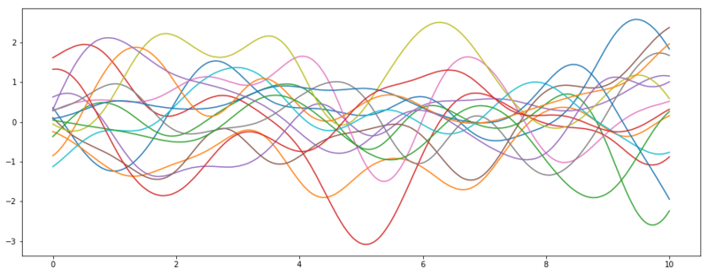
Samples from the prior distribution of $f_*$
Posterior probability
mean
Now we will find the mean and covariance matrix for the posterior. Let’s start with the mean $\mu_*$.
$$ \mu_* = k_*^T \alpha $$
Where $\alpha = (L^T)^{-1} \cdot L^{-1}f$, $L = \text{cholesky}(k + \sigma_n^2 I)$, and $\sigma_n^2$ is the noise in the observations (can be close to zero for noise-less regression).
# find mean mu*
K = kernel(x, x, l=0.9)
K_s = kernel(x, x_s, l=0.9)
L = np.linalg.cholesky(K + 1e-6 * np.eye(len(x)))
alpha = np.linalg.solve(L.T, np.linalg.solve(L, f(x)))
mu = K_s.T @ alpha
covariance
The covariance matrix is defined by
$$\Sigma_* = k_{**} - v^Tv$$
where $v = L^{-1} k_*$.
# determine covariance matrix
v = np.linalg.solve(L, K_s)
variance = K_ss - v.T @ v
Let $B = \text{cholesky}(\Sigma_* + \sigma_n^2 I)$ and we can sample from the posterior by
$$ p(f_*|f) = \mu_* + B \mathcal{N}(0, I)$$
# Sample 10 functions from the posterior
B = np.linalg.cholesky(variance + 1e-6 * np.eye(variance.shape[0]))
f_post = mu[:, None] + B @ np.random.normal(size=(n, 10))

# Find standard deviation for plotting uncertainty values.
s2 = np.ones(n) - np.sum(v**2, axis=0)
std = np.sqrt(s2)

plt.figure(figsize=(12, 6))
plt.plot(x, f(x), 'bs', ms=8, color='red')
plt.plot(x_s, f_post)
plt.fill_between(x_s, mu - 2 * std, mu + 2 * std, color="#dddddd")
plt.plot(x_s, mu, 'r--', lw=2)
plt.show()
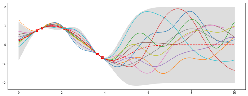
10 samples from the posterior
In the plot above we see the result from our posterior distribution. We sample functions that fit our training data (the red squares). So the amount of possible infinite functions that could describe our data has been reduced to a lower amount of infinite functions [if that makes sense ;)]. It is also very nice that we get uncertainty boundaries are smaller in places where we have observed data and widen where we have not. For now, we did noiseless regressions, so the uncertainty is nonexistent where we observed data. We could generalize this example to noisy data and also include functions that are within the noise margin. The red dashed line shows the mean of the posterior and would now be our best guess for $f(x)$.
This post was an introduction to Gaussian processes and described what it meant to express functions as samples from a distribution. I hope it gave some insight into the abstract definition of GPs. You may also take a look at Gaussian mixture models where we utilize Gaussian and Dirichlet distributions to do nonparametric clustering.