
In the posts Expectation Maximization and Bayesian inference; How we are able to chase the Posterior, we laid the mathematical foundation of variational inference. This post we will continue on that foundation and implement variational inference in Pytorch. If you are not familiar with the basis, I’d recommend reading these posts to get you up to speed.
This post we’ll model a probablistic layer as output layer of a neural network. This will give us insight in the aleatoric uncertainty (the noise in the data). We will evaluate the results on a fake dataset borrowed from this post.
import numpy as np
import torch
from torch import nn
from sklearn import datasets
import matplotlib.pyplot as plt

w0 = 0.125
b0 = 5.
x_range = [-20, 60]

def load_dataset(n=150, n_tst=150):
    np.random.seed(43)

    def s(x):
        g = (x - x_range[0]) / (x_range[1] - x_range[0])
        return 3 * (0.25 + g**2.)

    x = (x_range[1] - x_range[0]) * np.random.rand(n) + x_range[0]
    eps = np.random.randn(n) * s(x)
    y = (w0 * x * (1. + np.sin(x)) + b0) + eps
    y = (y - y.mean()) / y.std()
    idx = np.argsort(x)
    x = x[idx]
    y = y[idx]
    return y[:, None], x[:, None]

y, x = load_dataset()
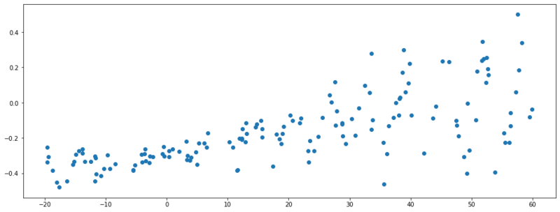
Generated data with noise dependent on $X$.
Maximum likelihood estimate
First we’ll model a neural network $g_{\theta}(x)$ with maximum likelihood estimation. Where we assume a Gaussian likelihood.
$$\begin{equation} y \sim \mathcal{N}(g_{\theta}(x), \sigma^2) \end{equation}$$
# Go to pytorch world
X = torch.tensor(X, dtype=torch.float)
Y = torch.tensor(Y, dtype=torch.float)

class MaximumLikelihood(nn.Module):
    def __init__(self):
        super().__init__()
        self.out = nn.Sequential(
            nn.Linear(1, 20),
            nn.ReLU(),
            nn.Linear(20, 1)
        )
    def forward(self, x):
        return self.out(x)

epochs = 200
m = MaximumLikelihood()
optim = torch.optim.Adam(m.parameters(), lr=0.01)

for epoch in range(epochs):
    optim.zero_grad()
    y_pred = m(X)
    loss = (0.5 * (y_pred - Y)**2).mean()
    loss.backward()
    optim.step()
If we train this model, we might observe a regression line like below. We are able to predict the expectation of y, but we are not able to make a statement about the noise of our predictions. The outputs are point estimates.
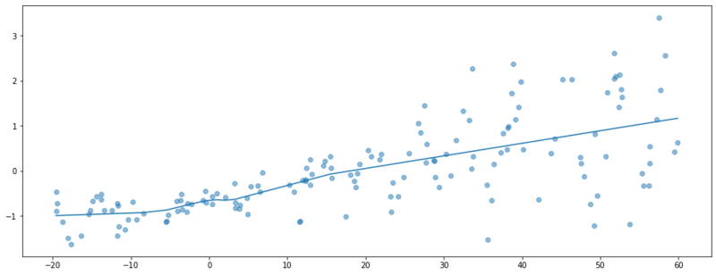
Fitted model with MLE.
Variational regression
Now let’s consider a model where we want to obtain the distribution $P(y|x) \propto P(x|y) P(y)$. In variational inference, we accept that we cannot obtain the true posterior $P(y|x)$, but we try to approximate this distribution with another distribution $Q_{\theta}(y)$, where $\theta$ are the variational parameters. This distribution we call a variational distribution.
If we choose a factorized (diagonal) Gaussian variational distribution, $Q_{\theta}(y)$ becomes $Q_{\theta}(\mu, \text{diag}(\sigma^2))$. Note that we are now working with an 1D case and that this factorization doesn’t mean much right now. We want this distribution to be conditioned to $x$, therefore we define a function $g_{\theta}: x \mapsto \mu, \sigma$. The function $g_{\theta}$ will be a neural network that predicts the variational parameters. The total model can thus be described as:
$$ \begin{equation}P(y) = \mathcal{N}(0, 1) \end{equation}$$
$$ \begin{equation}Q(y|x) = \mathcal{N}(g_{\theta}(x)_{\mu}, \text{diag}(g_{\theta}(x)_{\sigma^2})))\end{equation}$$
Where we set a unit Gaussian prior $P(y)$.
Optimization problem
Note: Above we’ve defined the posterior and the variational distribution in the variable $y|x$, from now on we will generalize to a notation that is often used. We’ll extend $y|x$ to any (latent) stochastic variable $Z$.
Variational inference is done by maximizing the ELBO (Evidence Lower BOund). Which is often written in a more intuitive form:
$$ \begin{equation}\text{argmax}_{Z} = E_{Z \sim Q}[\underbrace{\log P(D|Z)}_{\text{likelihood}}] - D_{KL}(Q(Z)||\underbrace{P(Z)}_{\text{prior}}) \label{eq:elbo} \end{equation}$$
Where we have a likelihood term (in Variational Autoencoders often called reconstruction loss) and the KL-divergence between the prior and the variational distribution. We are going to rewrite this ELBO definition so that it is more clear how we can use it to optimize the model, we’ve just defined.
Let’s first rewrite the KL-divergence term in integral form;
\begin{equation}E_{Z \sim Q}[\log P(D|Z)] + \int Q(Z) \frac{P(Z)}{Q(Z)}dZ \end{equation}
Note that the change of sign is due to the definition of the KL-divergence $D_{KL}(P||Q) = \int P(x) \log \frac{P(x)}{Q(x)}dx = -\int P(x) \log \frac{Q(x)}{P(x)}dx$.
Now we observe that we can rewrite the integral form as an expectation $Z$;
\begin{equation} E_{Z \sim Q}[\log P(D|Z)] + E_{Z \sim Q}[ \frac{P(Z)}{Q(Z)}]dZ \end{equation}
And by applying the log rule $\log\frac{A}{B}=\log A - \log B$, we get;
\begin{equation} E_{Z \sim Q}[\log P(D|Z)] + E_{Z \sim Q}[\log P(Z) - \log Q(Z) ] \end{equation}
Monte Carlo ELBO
Deriving those expectations can be some tedious mathematics, or maybe not even possible. Luckily we can get estimates of the mean by taking samples from $Q(Z)$ and average over those results.
Reparameterization trick
If we start taking samples from a $Q(Z)$ we leave the deterministic world, and the gradient can not flow through the model anymore. We avoid this problem by reparameterizing the samples from the distribution.
Instead of sampling directly from the variational distribution;
\begin{equation} z \sim Q(\mu, \sigma^2) \end{equation}
We sample from a unit gaussian and recreate samples from the variational distribution. Now the stochasticity of $\epsilon$ is external and will not prevent the flow of gradients.
\begin{equation} z = \mu + \sigma \odot \epsilon \end{equation}
Where
\begin{equation} \epsilon \sim \mathcal{N}(0, 1) \end{equation}
Implementation
This is all we need for implementing and optimizing this model. Below we’ll define the model in Pytorch. By calling the forward method we retrieve samples from the variational distribution.
class VI(nn.Module):
    def __init__(self):
        super().__init__()

        self.q_mu = nn.Sequential(
            nn.Linear(1, 20),
            nn.ReLU(),
            nn.Linear(20, 10),
            nn.ReLU(),
            nn.Linear(10, 1)
        )
        self.q_log_var = nn.Sequential(
            nn.Linear(1, 20),
            nn.ReLU(),
            nn.Linear(20, 10),
            nn.ReLU(),
            nn.Linear(10, 1)
        )

    def reparameterize(self, mu, log_var):
        # std can not be negative, thats why we use log variance
        sigma = torch.exp(0.5 * log_var) + 1e-5
        eps = torch.randn_like(sigma)
        return mu + sigma * eps

    def forward(self, x):
        mu = self.q_mu(x)
        log_var = self.q_log_var(x)
        return self.reparameterize(mu, log_var), mu, log_var
The prior, the likelihood and the varitational distribution are all Gaussian, hence we only need to derive the log likelihood function for the Gaussian distribution.
\begin{equation} \mathcal{L}(\mu, \sigma, x)= -\frac{n}{2}(2\pi \sigma^2) - \frac{1}{2\sigma^2}\sum_{i=1}^n(x_i - \mu)^2 \end{equation}
def ll_gaussian(y, mu, log_var):
    sigma = torch.exp(0.5 * log_var)
    return -0.5 * torch.log(2 * np.pi * sigma**2) - (1 / (2 * sigma**2))* (y-mu)**2
In the elbo function below, it all comes together. We compute the needed probabilities, and last we get an estimate of the expectation (see ELBO definition) by taking the means over a complete batch. In the det_loss function, we only reverse the sign, as all the optimizers in Pytorch are minimizers, not maximizers. And that is all we need, the result is an optimization problem with gradients. Hardly a problem at all in times of autograd.
def elbo(y_pred, y, mu, log_var):
    # likelihood of observing y given Variational mu and sigma
    likelihood = ll_gaussian(y, mu, log_var)

    # prior probability of y_pred
    log_prior = ll_gaussian(y_pred, 0, torch.log(torch.tensor(1.)))

    # variational probability of y_pred
    log_p_q = ll_gaussian(y_pred, mu, log_var)

    # by taking the mean we approximate the expectation
    return (likelihood + log_prior - log_p_q).mean()

def det_loss(y_pred, y, mu, log_var):
    return -elbo(y_pred, y, mu, log_var)
epochs = 1500

m = VI()
optim = torch.optim.Adam(m.parameters(), lr=0.005)

for epoch in range(epochs):
    optim.zero_grad()
    y_pred, mu, log_var = m(X)
    loss = det_loss(y_pred, Y, mu, log_var)
    loss.backward()
    optim.step()
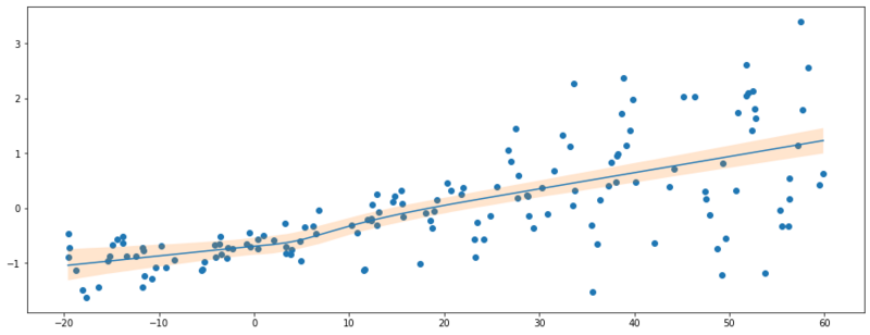
With the fitted model, we can draw samples from the approximate posterior. As we see in the plot below, the aleatoric uncertainty is incorporated in the model.
# draw samples from Q(theta)
with torch.no_grad():
    y_pred = torch.cat([m(X)[0] for _ in range(1000)], dim=1)

# Get some quantiles
q1, mu, q2 = np.quantile(y_pred, [0.05, 0.5, 0.95], axis=1)

plt.figure(figsize=(16, 6))
plt.scatter(X, Y)
plt.plot(X, mu)
plt.fill_between(X.flatten(), q1, q2, alpha=0.2)
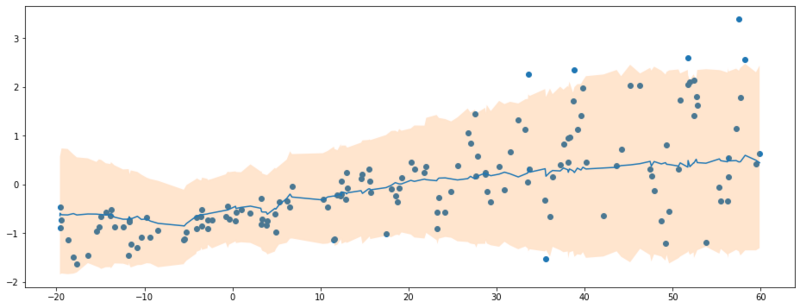
90% credible interval of $P(y|x)$.
Analytical KL-divergence and reconstruction loss
Above we have implemented ELBO by sampling from the variational posterior. It turns out that for the KL-divergence term, this isn’t necessary as there is an analytical solution. For the Gaussian case, Diederik P. Kingma and Max Welling (2013. Auto-encoding variational bayes) included the solution in Appendix B.
\begin{equation} D_{KL}(Q(Z)||P(Z)) = \frac{1}{2}\sum_{i=1}^n(1+\log \sigma_i^2 - \mu_i^2 - \sigma_i^2) \end{equation}
For the likelihood term, we did implement Guassian log likelihood, this term can also be replaced with a similar loss functions. For Gaussian likelihood we can use squared mean error loss, for Bernoulli likelihood we could use binary cross entropy etc. If we do that for the earlier defined model, we can replace the loss function as defined below:
def det_loss(y, y_pred, mu, log_var):
    reconstruction_error = (0.5 * (y - y_pred)**2).sum()
    kl_divergence = (-0.5 * torch.sum(1 + log_var - mu**2 - log_var.exp()))

    return (reconstruction_error + kl_divergence).sum()
Aleatoric and epistemic uncertainty
Update September 27, 2019
In the example above we have used variational inference to infer $y$ by setting an approximating distribution $Q_{\theta}(Y)$. Next we’ve defined a neural network capable of parameterizing this variational distribution $ f: \mathbb{R}^d \mapsto \mathbb{R}^n, \quad f(x) = \theta $, where $\theta = \{ \mu, \sigma \}$. By inherently modelling $\mu$ and $\sigma$ as a dependency on $X$, we were able to model the aleatoric uncertainty. This kind of uncertainty is called statistical uncertainty. This is the inherent variance in the data which we have to accept because the underlaying data generation process is stochastic in nature. In a pragmatic view, nature isn’t deterministic and some examples of random processes that lead to aleatoric uncertainty are:
- Throwing a dice.
- Firing an arrow with exactly the same starting conditions (the vibrations, wind, air pressure all may lead to a slightly different result).
- The cards you are dealt in a poker game.
Aleatory can have two flavors, being homoscedastic and heteroscedastic.
Homoscedastic
We often assume homoscedastic uncertainty. For example in the model definition of linear regression $y = X \beta + \epsilon$ we incorporate $\epsilon$ for the noise in the data. In linear regression, $\epsilon$ is not dependent on $X$ and is therefore assumed to be constant.
Example of homoscedastic uncertainty. [2]
Heteroscedastic
If the aleatoric uncertainty is dependent on $X$, we speak of heteroscedastic uncertainty. This was the case in the example we’ve used above. The figure below shows another example of heteroscedastic uncertainty.
Example of heteroscedastic uncertainty. [2]
Epistemic uncertainty
The second flavor of uncertainty is epistemic uncertainty. We as algorithm designers have influence on this type of uncertainty. We can actually reduce it, or make it much worse by our decisions. For instance, the way of bootstrapping the data when splitting test, train, and validation sets had influence on the parameters we fit. If we bootstrap differently, we end up with different parameter values, how certain can we be that these are correct? Epistemic uncertainty can be reduced by acquiring more data, designing better models, or by incorporating better features.
Bayes by backprop
In the next part of this post we’ll show an example of modelling epistemic uncertainty with variational inference. The implementation is according to this paper [3]. We will now be modelling the weights $w$ of the neural network with distributions. A priori, our bayesian model consists of the following prior and likelihood.
Again, the posterior $P(w|y, x)$ is intractable. So we define a variational distribution $Q_{\theta}(w)$. The theory of variational inference is actually exactly the same as we’ve defined in the first part of the post. For convenience reasons we redefine the ELBO as defined in (eq. $\ref{eq:elbo}$) in a form used in [3]. If we multiply the ELBO with $-1$, we obtain a cost function that is called the variational free energy.
\begin{equation} \mathcal{F(D, \theta)}= D_{KL}(Q(Z|\theta) || P(Z)) - E_{Z \sim Q}[\log P(D|Z)] \label{eq:vfe} \end{equation}
Single Bayesian layer
Just as with the model we have defined earlier, we will approximate all the terms in (eq. $\ref{eq:vfe}$) by sampling $z \sim Q(Z)$. The KL-divergence is not dependent on $D$, and can therefore be computed at the moment of sampling $z$. We will use this insight now as we will make a Bayesian neural network layer in pytorch.
class LinearVariational(nn.Module):
    """
    Mean field approximation of nn.Linear
    """
    def __init__(self, in_features, out_features, parent, n_batches, bias=True):
        super().__init__()
        self.in_features = in_features
        self.out_features = out_features
        self.include_bias = bias
        self.parent = parent
        self.n_batches = n_batches

        if getattr(parent, 'accumulated_kl_div', None) is None:
            parent.accumulated_kl_div = 0

        # Initialize the variational parameters.
        # 𝑄(𝑤)=N(𝜇_𝜃,𝜎2_𝜃)
        # Do some random initialization with 𝜎=0.001
        self.w_mu = nn.Parameter(
            torch.FloatTensor(in_features, out_features).normal_(mean=0, std=0.001)
        )
        # proxy for variance
        # log(1 + exp(ρ))◦ eps
        self.w_p = nn.Parameter(
            torch.FloatTensor(in_features, out_features).normal_(mean=-2.5, std=0.001)
        )
        if self.include_bias:
            self.b_mu = nn.Parameter(
                torch.zeros(out_features)
            )
            # proxy for variance
            self.b_p = nn.Parameter(
                torch.zeros(out_features)
            )

    def reparameterize(self, mu, p):
        sigma = torch.log(1 + torch.exp(p))
        eps = torch.randn_like(sigma)
        return mu + (eps * sigma)

    def kl_divergence(self, z, mu_theta, p_theta, prior_sd=1):
        log_prior = dist.Normal(0, prior_sd).log_prob(z)
        log_p_q = dist.Normal(mu_theta, torch.log(1 + torch.exp(p_theta))).log_prob(z)
        return (log_p_q - log_prior).sum() / self.n_batches

    def forward(self, x):
        w = self.reparameterize(self.w_mu, self.w_p)

        if self.include_bias:
            b = self.reparameterize(self.b_mu, self.b_p)
        else:
            b = 0

        z = x @ w + b

        self.parent.accumulated_kl_div += self.kl_divergence(w,
                                                             self.w_mu,
                                                             self.w_p,
                                                             )
        if self.include_bias:
            self.parent.accumulated_kl_div += self.kl_divergence(b,
                                                                 self.b_mu,
                                                                 self.b_p,
                                                                 )
        return z
The code snippet above shows the implementation of the variational linear layer. The __init__ method initializes the variation parameters $\mu_{w}$ and $p_{w}$. In the forward method we sample the weights $w \sim \mathcal{N}(\mu_{w}, \text{diag}(\log(1 + e^{p_w}) )$ and the biases $b \sim \mathcal{N}(\mu_{b}, \text{diag}(\log(1 + e^{p_b}) )$. With these sampled neural networks parameters we do the forward pass of that layer $z = xw + b$. As discussed, we also compute the KL-divergence in the forward method as we don’t require any target variable to determine this quantity.
KL re-weighting
When optimizing with stochastic gradient descent, the KL-divergence in term in (eq. $\ref{eq:vfe}$) needs to be weighed by $\frac{1}{M}$, where $M$ is the number of mini-batches per epoch.
Bayesian neural network
This LinearVariational is the gist of a Bayesian neural network optimized with variational inference. In the code snippet below, we implement the same network as before. The only difference in the previous implementation is an auxiliary dataclass that will accumulate the KL-divergences of the variational layers. The code snippets below shows the final implementation, the loss function and the train loop.
@dataclass
class KL:
    accumulated_kl_div = 0

class Model(nn.Module):
    def __init__(self, in_size, hidden_size, out_size, n_batches):
        super().__init__()
        self.kl_loss = KL

        self.layers = nn.Sequential(
            LinearVariational(in_size, hidden_size, self.kl_loss, n_batches),
            nn.ReLU(),
            LinearVariational(hidden_size, hidden_size, self.kl_loss, n_batches),
            nn.ReLU(),
            LinearVariational(hidden_size, out_size, self.kl_loss, n_batches)
        )

    @property
    def accumulated_kl_div(self):
        return self.kl_loss.accumulated_kl_div

    def reset_kl_div(self):
        self.kl_loss.accumulated_kl_div = 0

    def forward(self, x):
        return self.layers(x)
epochs = 2000

def det_loss(y, y_pred, model):
    batch_size = y.shape[0]
    reconstruction_error = -dist.Normal(y_pred, .1).log_prob(y).sum()
    kl = model.accumulated_kl_div
    model.reset_kl_div()
    return reconstruction_error + kl

m = Model(1, 20, 1, n_batches=1)
optim = torch.optim.Adam(m.parameters(), lr=0.01)

for epoch in range(epochs):
    optim.zero_grad()
    y_pred = m(X)
    loss = det_loss(y_pred, Y, m)
    loss.backward()
    optim.step()
Epistemic uncertainty
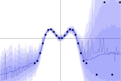
Below we evaluate the trained model by taking 1000 samples per data point. These samples are used to approximate quantities of the posterior predictive distribution such as the mean and the $\{0.05, 0.95 \}$ quantiles. Intuitively, we can think of each 1 of the 1000 samples as a different neural network with slightly different parameters.
with torch.no_grad():
    trace = np.array([m(X).flatten().numpy() for _ in range(1000)]).T
q_25, q_95 = np.quantile(trace, [0.05, 0.95], axis=1)
plt.figure(figsize=(16, 6))
plt.plot(X, trace.mean(1))
plt.scatter(X, Y)
plt.fill_between(X.flatten(), q_25, q_95, alpha=0.2)
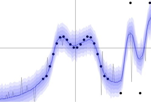
Results of the Bayesian neural network optimized w/ variation inference.
We see we didn’t model the aleatoric uncertainty. What we’ve captured now is the uncertainty of the true mean value, $E[Y|X]$.
Final words
This post we’ve implemented variational inference in two flavors. In one we’ve modelled aleatoric uncertainty and got insight in the changing variance of $y \sim P(Y|X)$. The second implementation was a fully bayesian neural network and resulted in epistemic uncertainty. In this implementation we were not interested in the uncertainty in the data, but in the uncertainty of our model. Variational inference seems to be a powerful, modular approach to enrich deep learning with uncertainty values.
I don’t believe I have to stress the importance of modeling uncertainty, yet in most machine learning models uncertainty is regarded secundary. Yu Ri Tan has got a very nice blog post on this topic. He explores how we can get insight in the uncertainty of our models in a frequentistic manner. Do read!
References
[1] Kingma & Welling (2013, Dec 20) Auto-Encoding Variational Bayes. Retrieved from https://arxiv.org/abs/1312.6114
[2] Gal, Y. (2016, Feb 18) HeteroscedasticDropoutUncertainty. Retrieved from https://github.com/yaringal/HeteroscedasticDropoutUncertainty
[3] Blundell, Cornebise, Kavukcioglu & Wierstra (2015, May 20) Weight Uncertainty in Neural Networks. Retrieved from https://arxiv.org/abs/1505.05424