
Not that long ago I wrote an introduction post on Gaussian Processes (GP’s), a regression technique where we condition a Gaussian prior distribution over functions on observed data. GP’s can model any function that is possible within a given prior distribution. And we don’t get a function $f$, we get a whole posterior distribution of functions $P(f|X)$.
This of course, sounds very cool and all, but there is no free lunch. GP’s have a complexity $\mathcal{O}(N^3)$, where $N$ is the number of data points. GP’s work well up to approximately 1000 data points (I should note that there are approximating solutions that scale better). This led me to believe that I wouldn’t be using them too much in real-world problems, but luckily I was very wrong!
Bayesian Optimization
This post is about bayesian optimization (BO), an optimization technique, that gains more tractions over the past few years, as its being used to search for optimal hyperparameters in neural networks. BO is actually a useful optimization algorithm for any black-box function that is costly to evaluate. Black box, in this sense, means that we observe only the (noisy) outputs of the function and not more information that could be to our advantage (i.e. first- or second-order derivatives). By ‘costly’, we mean that the function evaluations are on a certain budget. There are resources required to evaluate the function. These resources are often time or money.
Some examples where bayesian optimization can be useful are:
- Hyperparameter search for machine learning
- Parameter search for physics models
- Calibration of environmental models
- Increasing conversion rates
These subjects are time-consuming, have a large parameter space, and the implementations are ‘black-box’ as we can’t compute derivatives.
Some examples where you shouldn’t use Bayesian Optimization:
- Curve fitting
- Linear programming
For these kinds of problems, there are better optimization algorithms that can, for instance, take advantage of the shape of the function’s codomain (convex problems).
This post we are going to implement a Bayesian Optimization algorithm in Python and while doing so we are going to explore some properties of the algorithm.
Why Gaussian Processes?
Bayesian optimization is thus used to model unknown, time-consuming to evaluate, non-convex, black-box functions $f$. Let’s think for a moment about some of the properties we would want for such a model.
Exploration
Most models fit in a frequentist manner and lead to a point estimate of the parameters that best fit the function. Once we’ve fitted a model on $f(x)$, it is hard to get a sense of the uncertainty of our model. We want to have a notion of uncertainty because we don’t want to explore a space where we are very certain and we already know what the outcome will be. This would be a waste of our limited budget. So we want to be able to do exploration and for that, we need to know the uncertainty, i.e. we need Bayesian models. On to the second requirement!
Versatility
As BO is useful for any black-box function (which can have any output shape), we do need a versatile model to be able to approximate the unknown black-box function. For this reason, we can’t use linear or polynomial regression as we restrict our model to a certain function family. Gaussian Processes fit this requirement. We can just set a prior distribution over functions and with a kernel, we can restrict (or not) the family of possible functions as much as we want.
The limiting scalability properties of GP’s now actually don’t matter as the function evaluations are on a limiting budget. Every new data point is costly, so we’ll stay well below 1000 data points!
The algorithm
Below the BO algorithm is shown in pseudo-code. Later we will implement in Python.
Place prior over f.

Define an acquisition function that given a posterior
distribution determines new sample locations.

Evaluate n random samples of f.

while i < budget do:
   Determine posterior distribution conditioned on the current samples of f.

   Find new parameters X_i by maximizing the acquisition function.

   Evaluate f(X_i) and store output.

   Increment i.
Expected Improvement
In the pseudo-code example we define an acquisition function. The acquisition function can be any function that reflects the location we want to evaluate next. A function that is often used is called Expected Improvement;
$$\text{EI}(x) = \mathbb{E}\max(f(x^*) - f(x^+), 0)$$
Where $x^*$ are the proposal parameters, and $x^+$ are the current highest evaluated parameters. This expectation has a closed form solution defined by;
$$\text{EI}(x) = \delta \Phi(Z) + \sigma(x^*) \phi(Z)$$
Where $\delta = \mu(x^*) - f(x^+)$ and
Note that $\Phi$ and $\phi$ are the CDF and PDF of a unit Gaussian distribution, respectively.
See this blog post for the derivation.
In Python we can easily implement this acquisition function.
# our imports for today
import numpy as np
import GPy
from scipy import stats
from scipy import optimize
from tqdm import tqdm
from functools import partial
import matplotlib.pyplot as plt

def expected_improvement(f, y_current, x_proposed):
    """
    Return E(max(f_proposed - f_current), 0)

    Parameters
    ----------

    f : GP predict function
    y_current : float
        Current best evaluation f(x+)
    x_proposed : np.array
        Proposal parameters. Shape: (1, 1)

    Returns
    -------
    expected_improvement : float
        E(max(f_proposed - f_current), 0)
    """
    mu, var = f(x_proposed)
    std = var ** 0.5
    delta = mu - y_current

    # x / inf = 0
    std[std == 0] = np.inf
    z = delta / std
    unit_norm = stats.norm()
    return delta * unit_norm.cdf(z) + std * unit_norm.pdf(z)
Bayesian Optimization Implementation
Below we will define the BO algorithm from scratch, except for the Gaussian Processes. For the GP’s we’ll use GPy by SheffieldML. If you want to a quick tutorial on how to implement a GP in GPy, take a look at this jupyter notebook. In the directory above there are more implementations, such as a GP from scratch and a GP in PymC3.
Utility functions
Besides an expected_improvement function, we’ll define another utility function for selecting hyperparameters at a given hyperparameter range at random.
def select_hyperparams_random(param_ranges):
    """
    Select hyperparameters at random.

    Parameters
    ----------
    param_ranges : dict
        Named parameter ranges.

        Example:

        {
            'foo': {
                'range': [1, 10],
                'type': 'float'
            }
            'bar': {
                'range': [10, 1000],
                'type': 'int'
            }
        }

    Returns
    -------
    selection : dict
        Randomly selected hyperparameters within given boundaries.

        Example:
        {'foo': 4.213, 'bar': 935}

    """
    selection = {}
    for k in param_ranges:
        val = np.random.choice(np.linspace(*param_ranges[k]["range"], num=100))

        dtype = param_ranges[k]["type"]
        if dtype is "int":
            val = int(val)
        selection[k] = val
    return selection
See the docstring for the input and outputs given by this function.
Bayesian Optimization class
These are all the utility functions we need. Now we can implement the whole Bayesian Optimization model. For reading purposed the whole implementation is shown at once. Below the code snippet, we’ll go through some methods of this class to get an understanding of what we are doing.
class BayesOpt:
    def __init__(
        self, param_ranges, f, random_trials=5, optimization_trials=20, kernel=None
    ):
        """
        Parameters
        ----------

        param_ranges : dict
        f : function
            black box function to evaluate
        random_trials : int
            Number of random trials to run before optimization starts
        optimization_trials : int
            Number of optimization trials to run.
            Together with the random_trials this is the total budget
        kernel: GPy.kern.src.kern.Kern
            GPy kernel for the Gaussian Process.
            If None given, RBF kernel is used
        """
        self.param_ranges = param_ranges
        self.f = f
        self.random_trials = random_trials
        self.optimization_trials = optimization_trials
        self.n_trials = random_trials + optimization_trials
        self.x = np.zeros((self.n_trials, len(param_ranges)))
        self.y = np.zeros((self.n_trials, 1))

        if kernel is None:
            self.kernel = GPy.kern.RBF(
                input_dim=self.x.shape[1], variance=1, lengthscale=1
            )
        else:
            self.kernel = kernel
        self.gp = None
        self.bounds = np.array([pr["range"] for pr in param_ranges.values()])

    @property
    def best_params(self):
        """
        Select best parameters.

        Returns
        -------
        best_parameters : dict
        """
        return self._prepare_kwargs(self.x[self.y.argmax()])

    def fit(self):
        self._random_search()
        self._bayesian_search()

    def _random_search(self):
        """
        Run the random trials budget
        """
        print(f"Starting {self.random_trials} random trials...")
        for i in tqdm(range(self.random_trials)):
            hp = select_hyperparams_random(self.param_ranges)
            self.x[i] = np.array(list(hp.values()))
            self.y[i] = self.f(hp)

    def _bayesian_search(self):
        """
        Run the Bayesian Optimization budget
        """
        print(f"Starting {self.optimization_trials} optimization trials...")
        for i in tqdm(
            range(self.random_trials, self.random_trials + self.optimization_trials)
        ):
            self.x[i], self.y[i] = self._single_iter()

    def _single_iter(self):
        """
        Fit a GP and retrieve and evaluate a new
        parameter proposal.

        Returns
        -------
        out : tuple[np.array[flt], np.array[flt]]
            (x, f(x))

        """
        self._fit_gp()
        x = self._new_proposal()
        y = self.f(self._prepare_kwargs(x))
        return x, y

    def _fit_gp(self, noise_var=0):
        """
        Fit a GP on the currently observed data points.

        Parameters
        ----------
        noise_var : flt
            GPY argmument noise_var
        """
        mask = self.x.sum(axis=1) != 0
        self.gp = GPy.models.GPRegression(
            self.x[mask],
            self.y[mask],
            normalizer=True,
            kernel=self.kernel,
            noise_var=noise_var,
        )
        self.gp.optimize()

    def _new_proposal(self, n=25):
        """
        Get a new parameter proposal by maximizing
        the acquisition function.

        Parameters
        ----------
        n : int
            Number of retries.
            Each new retry the optimization is
            started in another parameter location.
            This improves the chance of finding a global optimum.

        Returns
        -------
        proposal : dict
            Example:
           {'foo': 4.213, 'bar': 935}
        """

        def f(x):
            return -expected_improvement(
                f=self.gp.predict, y_current=self.y.max(), x_proposed=x[None, :]
            )

        x0 = np.random.uniform(
            low=self.bounds[:, 0], high=self.bounds[:, 1], size=(n, self.x.shape[1])
        )
        proposal = None
        best_ei = np.inf
        for x0_ in x0:
            res = optimize.minimize(f, x0_, bounds=self.bounds)
            if res.success and res.fun < best_ei:
                best_ei = res.fun
                proposal = res.x
            if np.isnan(res.fun):
                raise ValueError("NaN within bounds")
        return proposal

    def _prepare_kwargs(self, x):
        """
        Create a dictionary with named parameters
        and the proper python types.

        Parameters
        ----------
        x : np.array
            Example:
            [4.213, 935.03]

        Returns
        -------
        hyperparameters : dict

            Example:
            {'foo': 4.213, 'bar': 935}
        """
        # create hyper parameter dict
        hp = dict(zip(self.param_ranges.keys(), x))
        # cast values
        for k in self.param_ranges:
            if self.param_ranges[k]["type"] == "int":
                hp[k] = int(hp[k])
            elif self.param_ranges[k]["type"] == "float":
                hp[k] = float(hp[k])
            else:
                raise ValueError("Parameter type not known")
        return hp
I will go through some of the methods. Not all as most will be self-explanatory (I hope).
__init__(self)
Here we instantiate the BayesOpt model. We’ll set some attributes we’ll need for the model. It is important to note that we pass f here. This is the black box function we want to approximate. Furthermore, we set the number of random_trials and optimization_trials here. The sum of those is the total budget of function evaluations we may use.
__single_iter(self)
This is the method where we do a single Bayesian Optimization iteration. It consists of training a GP on the data points we’ve observed thus far. Then we pass this GP to the acquisition function and obtain a new parameter proposal by maximizing the acquisition function. With this new proposal $x^*$ we evaluate $f(x^*)$ and save the results.
_new_proposal(self, n)
In this method, we actually maximize the $EI(x)$ function. We’ll use scipy for that, but many optimization algorithms can be used for this (don’t use Bayesian Optimization though, recursion induced stack-overflow ;) ). Note that we pass n as a parameter. This dictates how many times we should restart the optimization algorithm that maximizes $EI(x)$ from a different (random) starting point. This is to reduce the chance of proposing a solution that is a local optimum.
Okay, that was it. Now let’s take this baby for a spin!
1D examples
Let’s start with an example in 1D. This will give us a good feeling of how Bayesian Optimization uses GP’s and the acquisition function for exploration.
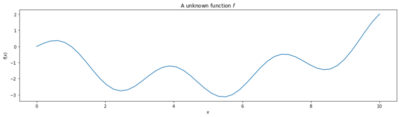
First we generate a multi model function over a range $(0, 10)$.
x = np.linspace(0, 10)

def func(x):
    return np.sin(2 * x) + (x / 3)**2 - x + 50

plt.figure(figsize=(16, 4))
plt.title('A unknown function $f$')
plt.xlabel('$x$')
plt.ylabel('$f(x)$')
plt.plot(x, func(x))
Then we define the boundaries of the input and the evaluation function.
def evaluate_params(hyperparams):
    return func(**hyperparams)

param_ranges = {
    'x': {
        'range': [0, 10],
        'type': 'float'
    }
}
With these we can instantiate the BayesOpt class. We set at least 2 random trials otherwise it is impossible to fit a Gaussian Process.
np.random.seed(3)
bo = BayesOpt(param_ranges, evaluate_params, random_trials=2)
Next we take 8 optimization iterations and plot the fitted GP (left) and $EI(x)$ over our domain $(0, 10)$ (right). We also plot the trials we already have observed. The random trials in red, and the trials that we took during the optimization in green. Finally, we plot the the new proposal point for the next iteration. This is the dashed vertical line.
bo._random_search()
bo._fit_gp()
new_proposal = bo._new_proposal()
x_, y_ = bo._single_iter(new_proposal)

for i in range(2, 10):
    new_proposal = bo._new_proposal()
    ei = expected_improvement(
        f=bo.gp.predict, y_current=bo.y.max(), x_proposed=x[:, None]
    )
    x_, y_ = bo._single_iter(new_proposal)
    bo.x[i], bo.y[i] = x_, y_

    quants = bo.gp.predict_quantiles(x[:, None], quantiles=(10, 90))
    mu, var = bo.gp.predict(x[:, None])

    plt.figure(figsize=(20, 4))
    plt.suptitle(f"Iteration {i - 1}")
    plt.subplot(1, 2, 1)
    plt.title("$f(x^*)$")
    plt.plot(x, mu, color="C0", label="Mean")
    plt.fill_between(
        x,
        quants[0].flatten(),
        quants[1].flatten(),
        alpha=0.15,
        edgecolor="C1",
        label="Confidence",
    )
    plt.scatter(
        bo.x[: bo.random_trials],
        bo.y[: bo.random_trials],
        color="r",
        label="random trials",
    )
    plt.xlim(x.min() - 1, x.max() + 1)
    mask = bo.x.sum(axis=1) != 0
    plt.scatter(
        bo.x[mask][bo.random_trials : -1],
        bo.y[mask][bo.random_trials : -1],
        color="g",
        label="BO trials",
    )

    plt.legend()
    plt.subplot(1, 2, 2)
    plt.title("$EI(x)$")
    plt.plot(x, ei, color="C1")
    plt.vlines(new_proposal, 0, ei.max(), linestyle="--", label="New proposal")
    plt.xlim(x.min() - 1, x.max() + 1)
    plt.legend()
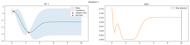
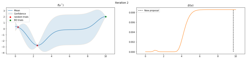
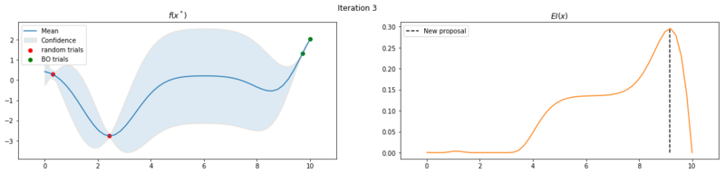
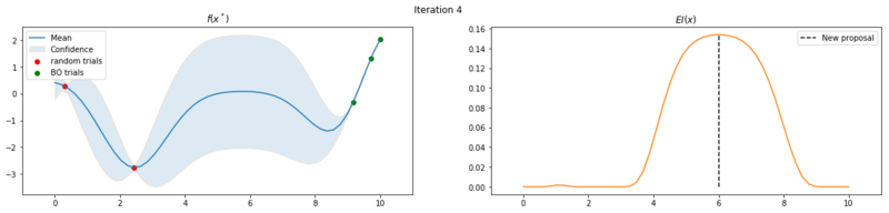
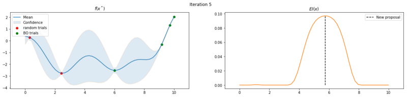
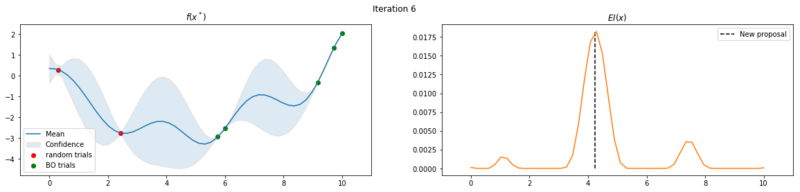
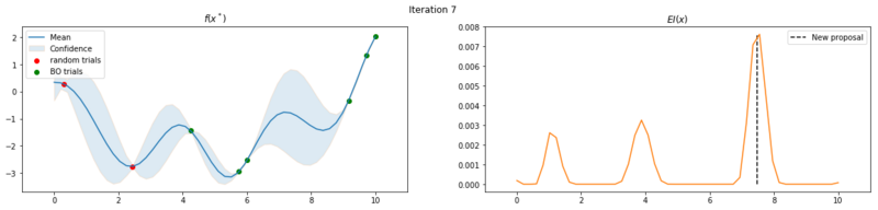
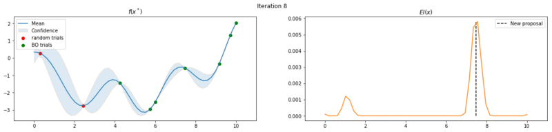
Explore the uncertainty by maximizing $EI(x)$
What is interesting to note, is that $EI(x)$ is not high in area’s we’ve already observed, It really favors unobserved areas that maximize the probability of increasing $f(x)$, hence Expected Improvement. If we continue the optimization we will be certain over the whole range $f(x)$ and $EI(x)$ will be close to zero for the whole range. Which reflects what we want, as we have a limited budget, there is no use in testing something we know the outcome of. The exploration characteristics of $EI(x)$ can clearly be seen in the figure below, which depicts the relation between $\delta = \mu(x^*) - f(x^+)$ and $\sigma(x^*)$.
delta = np.linspace(0, 1)
sigma = np.linspace(0, 1)[::-1]
# get a square grid w/ the delta and sigma inputs
dd, ss = np.meshgrid(delta, sigma)

# this is just the EI function
z = dd / ss
unit_norm = stats.norm()
ei = dd * unit_norm.cdf(z) + ss * unit_norm.pdf(z)
ei[np.isnan(ei)] = 0

plt.figure(figsize=(7, 7))
plt.title('$EI(x)$')
plt.contourf(delta, sigma, ei)
plt.xlabel('$\delta$')
plt.ylabel('$\sigma(x^*)$')
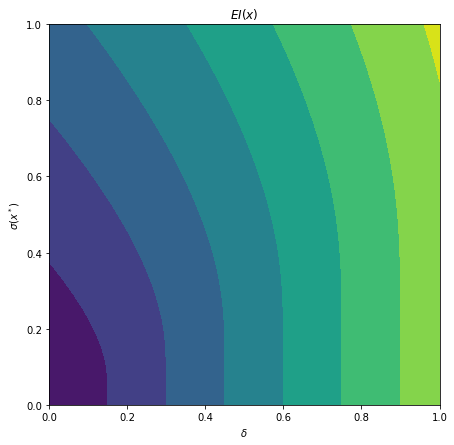
Exploration characteristics of $EI(x)$. $EI(x)$ is high where both the uncertainty $\sigma(x^*)$ and the improvement $\delta$ are high.
We can also observe that our proposal algorithm isn’t perfect, as the proposal of the first iteration is a local optimum. This isn’t too worrying as that point would probably a global optimum in a later iteration and it helps the GP with extra data points.
Higher dimensions
Bayesian optimization is of course not limited to 1D input. In this notebook I have an example of how we could use Bayesian Optimization to find more optimal solutions for a structural engineering problem. For an introduction to the problem, you can check this post.
A word about kernels
Kernels restrict the prior distribution of functions. A standard kernel is the Radius Basis Function kernel (RBF), which results in ‘smooth’ functions. It ensures that values, that are relatively close in the domain of $f$ are also relatively close in the codomain $f(x)$. This isn’t always a sensible default. In a step function, for instance, we have huge steps at a small change of $x$.
Kernels can also be combined, where multiplying can be seen as an AND operation and addition as an OR operation. There are a lot of kernels with different properties. I’d recommend taking a look at this kernel cookbook to get a concise overview.
Further reading and Implementations
This post we looked at how Bayesian Optimization can be used to optmize black box models. We’ve implemented BO in Python using GPy for the Gaussian Processes, and we’ve seen how Expected Improvement leads to exploring uncertain areas in of our black box function’s output.
Want to read more about Bayesian Optimization? Take a look at the following posts/ papers:
- Constrained Bayesian Optimization with NoisyExperiments (Letham et al.)
- Excellent blog post by Martin Krasser
- A Tutorial on Bayesian Optmization (Peter Frazier)
Some implementations of Bayesian Optimization are: