Frames
One of my first packages in Python is a program for analysing 2D Frames called anaStruct. I wrote this in the summer of 2016 and learned a lot by doing so. When it was ‘finished’ I was really enthusiastic and eager to give it some purpose in the ‘real’ engineering world.
My enthusiasm wasn’t for long though. I wrote a fem package that can compute linear force lines. The real world however isn’t so linear. The engineering problems in which linear fem packages are sufficient, most of the times aren’t the problems I am really interested in. Thus my first Python library was untouched for almost a year.
Problem
When I came across a water accumulation problem at work, my enthusisasm was reignited.
The frame shown in the figure below has got properties that aren’t easily modelled in standard frames software, or the software doesn’t support water accumulation analysis. The problem motivated me to update my old work and make anaStruct usable in the real world.
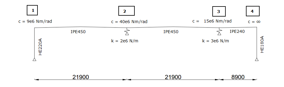
Frame.
The figure above shows a frame that is situated every 5 m. It has two IPE450 girders that span 21.9 m and a smaller IPE240 girder which spans 8.9 m. At axes 2 and 3 the beams are supported on two beams spanning in the perpendicular direction. This effect is modelled with two translational supported springs. Every steel member connection needs to be modelled with a rotational spring as the connections aren’t fully moment resisting, except for the connection of the steel member and the column on axis 4. The spring stiffnesses are shown in the figure. The bending moment capacity of the connections per axes are shown below.
- Moment axis 1: 70 kNm
- Moment axis 2: 240 kNm
- Moment axis 3: 25 kNm
- Moment axis 4: equal to the capacity of the HE180A column
The yield stress of the steel is equal to 235 MPa.
## Ponding rainwater Ok, now we've dealt with the specifications of the frame, we can discuss the problem at hand. The frame is part of a one layered structure. The IPE members of the frame are therefore part of the roof structure. If we look at the figure, we can see that there is a little bit of a slope in the beams. This must ensure that the water will run-off to the gutter, which are situated near the supports at axes 2 and 3. The essence of ponding (water accumulation) is the following. If we neglect the strength of the structure, the roof has a water storage capacity that is dependent of the shape of the roof and the height of the roofs edges. If we fill the roof with water until the maximum storage capacity is reached, the water level will be equal to height of the roof edge. However due to the weight of the water, the roof structure will deflect and by doing so increases the maximum storage capacity. If the water level remains constant, this effect can be thought of as an iterative process with two possible outcomes.
- The additional deflection due to the extra storage capacity will eventualy be neglectible, with amount of storaged water reaching an asymptote.
- The additional deflection increases every iteration, leading to more water weight untill the structure fails. The failure however isn’t because it is a strength problem, but because it is inevitable as the weight keeps increasing.
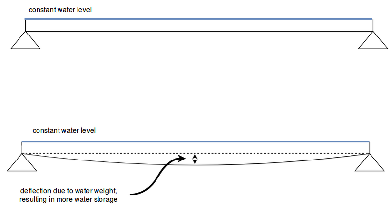
Accumulating water on a simple supported beam.
The first outcome is a bit like Zeno’s paradoxes. Every iteration the deflection will increase slightly, but it will eventually be such an infinitesimal small increase that failure will never occur. In the second outcome the deflection eventually increases every iteration, somewhat like Achilles actually overtaking the tortoise.
Just like buckling problems, water accumulation problems are stiffness problems. Failure due to too less strength capacity is just one of the possible outcomes due to a stiffness shortage.
## Upgrades In this post we are going to determine the maximum water storage capacity of this structure with nothing more than Python. Before being able to do so, anaStruct needed a few more functionalities. In order to be able to analyse this structure in Python I needed to meet up to the following requirements:
- force analysis
- displacement analysis
- supports with different degrees of freedom
- spring supports
- rotational spring elements
- nonlinear nodes
- q-loads in the global y-axis direction
- point-loads in global y-axis direction
How this was implemented could be a subject of another post, but after a few days and some shower epiphanies most the stated requirements were met and I can happily say that anaStruct is much more applicable in ‘real’ world problems than it was.
## Modelling the structure In the following section we are going to setup the code needed for a water accumulation analysis. The instalation instructions can be found at [Github](https://github.com/ritchie46/anaStruct). You can install the package using git. If you are on a windows machine, you'll need a git batch environment, which can be [downloaded here](https://git-scm.com/download/win).
In the code snippet below, we’ll import the required modules, functions and classes.
# import dependencies
import matplotlib.pyplot as plt
from anastruct.basic import converge
from anastruct.material.profile import HEA, IPE
from anastruct.fem.system import SystemElements, Vertex
from anastruct.material.units import to_kNm2, to_kN

# constants
E = 2.1e5  # Construction steels Young's modulus
b = 5  # c.t.c distance portals
q_water = 10

# axes height levels
h_1 = 0
h_2 = 0.258
h_3 = 0.046
h_4 = 0.274
h_5 = 0.032
h_6 = 0.15

# beam spans
span_1 = span_2 = 21.9
span_3 = 8.9

# Vertices at the axes
p1 = Vertex(0, h_1)
p2 = Vertex(span_1 * 0.5, h_2)
p3 = Vertex(span_1, h_3)
p4 = Vertex(span_1 + span_2 * 0.5, h_4)
p5 = Vertex(span_1 + span_2, h_5)
p6 = Vertex(span_1 + span_2 + span_3, h_6)
We import some helper functions and the SystemElements class. With this class’ objects we’re going to model the structure. The Vertex class produces objects that are, well, vertices.
After we’ve imported the dependencies, we’re defining some constants like the Young’s modules of the steel and the Vertices of the member joints at the axes 1 - 4. The vertices refer to the following locations:
p1: axis 1p2: between axis 1 and 2p3: axis 2p4: between axis 2 and 3p5: axis 3p6: axis 6
Next we’ll define a function structure() that we can call to model the portal. Later on we’ll see why we need to call the structure() function multiple times. The definition of the function is shown below.
def structure():
    """
    Build the structure from left to right, starting at axis 1.

    variables:
    EA = Young's modulus * Area
    EI = Young's modulus * moment of Inertia
    g = Weight [kN/ m]
    elements = reference of the element id's that were created
    dl = c.t.c distance different nodes.
    """

    dl = 0.2


    ## SPAN 1 AND 2

    # The elements between axis 1 and 3 are an IPE 450 member.
    EA = to_kN(E * IPE[450]['A'])  # Y
    EI = to_kNm2(E * IPE[450]["Iy"])
    g = IPE[450]['G'] / 100

    # New system.
    ss = SystemElements(mesh=3, plot_backend="mpl")

    # span 1
    first = dict(
        spring={1: 9e3},
        mp={1: 70},
    )

    elements = ss.add_multiple_elements(location=[p1, p2], dl=dl, first=first, EA=EA, EI=EI, g=g)
    elements += ss.add_multiple_elements(location=p3, dl=dl, EA=EA, EI=EI, g=g)

    # span 2
    first = dict(
        spring={1: 40e3},
        mp={1: 240}
    )
    elements += ss.add_multiple_elements(location=p4, dl=dl, first=first, EA=EA, EI=EI, g=g)
    elements += ss.add_multiple_elements(location=p5, dl=dl, EA=EA, EI=EI, g=g)


    ## SPAN 3

    # span 3
    # different IPE
    g = IPE[240]['G'] / 100
    EA = to_kN(E * IPE[240]['A'])
    EI = to_kNm2(E * IPE[240]["Iy"])
    first = dict(
        spring={1: 15e3},
        mp={1: 25},
    )

    elements += ss.add_multiple_elements(location=p6, first=first, dl=dl, EA=EA, EI=EI, g=g)

    # Add a dead load of -2 kN/m to all elements.
    ss.q_load(-2, elements, direction="y")


    ## COLUMNS

    # column height
    h = 7.2

    # left column
    EA = to_kN(E * IPE[220]['A'])
    EI = to_kNm2(E * HEA[220]["Iy"])
    left = ss.add_element([[0, 0], [0, -h]], EA=EA, EI=EI)

    # right column
    EA = to_kN(E * IPE[180]['A'])
    EI = to_kNm2(E * HEA[180]["Iy"])
    right = ss.add_element([p6, Vertex(p6.x, -h)], EA=EA, EI=EI)


    ## SUPPORTS

    # node ids for the support
    id_left = max(ss.element_map[left].node_map.keys())
    id_top_right = min(ss.element_map[right].node_map.keys())
    id_btm_right = max(ss.element_map[right].node_map.keys())

    # Add supports. The location of the supports is defined with the nodes id.
    ss.add_support_hinged((id_left, id_btm_right))

    # Retrieve the node ids at axis 2 and 3
    id_p3 = ss.find_node_id(p3)
    id_p5 = ss.find_node_id(p5)

    ss.add_support_roll(id_top_right, direction=1)

    # Add translational spring supports at axes 2 and 3
    ss.add_support_spring(id_p3, translation=2, k=2e3, roll=True)
    ss.add_support_spring(id_p5, translation=2, k=3e3, roll=True)
    return ss
Span 1 and span 2
First we define the properties of the IPE 450 girders between axes 1 and 3. Here we use to helper functions to_kN() and to_kNm() to ensure the right units. I haven’t mentioned it yet, but the units we are using are metrics:
- length: m
- force: kN
As the software is just nummerical, the imperical units should work just the same. We instantiate a variable called ss from the SystemElements class. Note that the mesh argument has no influence on the numerical result, but only on the plotters accuracy.
Next we use the .add_multiple_elements() method to add, ehh.. you’ll get the point. The iterator we pass as first arguments describes the two outer vertices. The dl arguments defines the distance the generated nodes. The total amount of generated nodes \( n \) is equal to:
Note that we also pass a dictionary first as argument. The method .add_multiple_elements() accepts a first and a last keyword argument describing deviating properties of the first or last elements.
The properties passed through this method are assigned to all elements, except if they differ in the first or last keyword argument. In our case we want to assign a rotational spring and a limited bending moment capacity to the first node (axis 1). Note that the keys of the dictionaries assigned to spring and mp refer to the elements nodes.
spring: Adds a rotational spring at the end of the element.mp: Adds a maximum bending moment capacity at the end of the element.
We assign the result of .add_multiple_elements() to a list variable we call elements. This list contains the IDs of the elements we just added. Every modelled element and node will have an unique ID. We need these IDs if we want to model load or support conditions.
Span 3
For span 3, between axes 3 and 4, the same principle as stated above is repeated. The properties of the beams were changed because the girder now is an IPE240 instead of an IPE450.
Now that all the girders are modelled we can apply a distributed load representing the weight of the roofing. This is done with the .q_load() method. As second argument we pass the elements list. Now we’ve applied a distributed load of 2 kN/m on all the elements.
columns
Then we add columns to the model. Both columns differ, so we change the properties EA and EI for both columns. Because we don’t need any intermediate node we can add the columns with the ss.add_element() method, which just adds one single element.
supports
In the last part of the function we define the supporting conditions of the model. We query the node IDs of the columns and assign those to id_left, id_top_right and id_btm_right. Those node IDS are passed to the self-explanatory called methods .add_support_roll() and .add_support_spring(). Which wraps up our structure function!
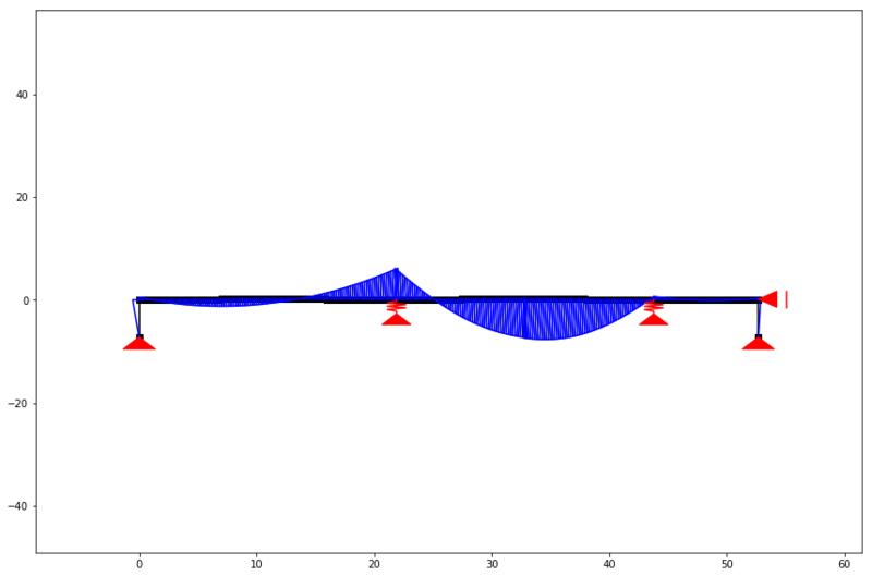
We can now take a look at the result of our model by calling the structure() function, retrieving a new SystemElement object and call the .show_structure() method!
ss = structure()
ss.show_structure(verbosity=1, scale=0.6)
This will plot the figure shown below. It is the same mechanical scheme we saw a the top of this post. The red patches show the support conditions and the green rectangles are the dead load applied on the structure.
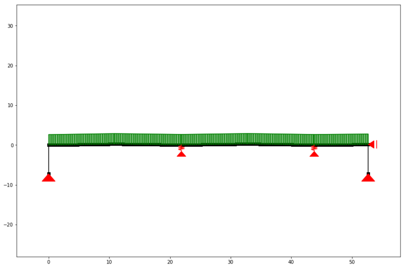
The model with a q-load of 2 kN/m
## Water loads The function we've just created will return the same model with the same q-load every time we call it. This is okay, as we don't want that the q-load changes during the iteration. What does change, when we talk about the concept of accumulating water is of course the water load. Therefore we need another function that will apply water loads on the structure. The water loads that are acting on the structure will depend on two factors, namely the water level and the amount of deflection the structure has that iteration.
We are going to model the water loads as point loads acting on the structure. This is the reason we’ve added so many nodes in the structure() function! The more nodes we model, the more accurate our analysis becomes.
def water_load(ss, water_height, deflection=None):
    """
    :param ss: (SystemElements) object.
    :param water_height: (flt) Water level.
    :param deflection: (array) Computed deflection.
    :return (flt) The cubic meters of water on the structure
    """

    # The horizontal distance between the nodes.
    dl = np.diff(ss.nodes_range('x'))

    if deflection is None:
        deflection = np.zeros(len(ss.node_map))

    # Height of the nodes
    y = np.array(ss.nodes_range('y'))

    # An array with point loads.
    # cubic meters * weight water
    force_water = (water_height - y[:-3] - deflection[:-3]) * q_water * b * dl[:-2]

    cubics = 0
    n = force_water.shape[0]
    for k in ss.node_map:
        if k > n:
            break
        point_load = force_water[k - 1]

        if point_load > 0:
            ss.point_load(k, Fx=0, Fz=-point_load)
            cubics += point_load / q_water

    return cubics
In the function above we compute the point loads resulting from a water level and an occurring deflection. We index with -3 because we are not interested in the last 4 nodes, as those are from the modelled columns. The -2 index is because we loose one value by differentiating an array. In the loop we do a final sanity check and only apply the positive point loads on the structure.
If we call this function and show the structure again, we can see that it mimics a water pressure with discrete point loads. The figure below really shows the influence of the roofs slope. It isn’t hard to imagine that the deflection may also have such an impact on the water load.
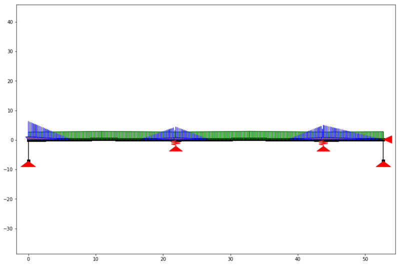
The model with a q-load of 2 kN/m and a water load of 150 mm.
## Iteration Now the model is ready and we can apply various water loads on this model, we can almost start with the iterative water accumulation analysis. Before doing so we must think about how we can do this iteration.
I think we’ve got two valid options to find the maximum water storage capacity:
- Apply a constant water level and keep iterating until the amount water stored in the roof converges to a constant level. Or it doesn’t and we should break the iteration and try another water level.
- Apply a constant water volume. This means that with every iteration we need to redistribute the water on the roof. You can think of this as a pool of water flowing to the lowest point. With this option the deflection will converge to a constant level.
In this post we are looking to the latter option, as this is gives a better view of the capacity of the structure. Because the deflection of the structure converges (resulting in a value of the water level) we can plot the volume of storaged water against the maximum water level. With such a diagram you’re able to find out if the drainage network of such a roof is capable processing these water volumes.
So if we implement the second option, we need a function that redistributes the water. The function below takes a volume c and an array of deflection values deflection. It will setup a new model of the structure with the proper water load applied. This model ss and the water level wh (for logging purposes) are returned.
The converge function takes a left hand side and a right hand side and returns a factor by which the left hand side should be multiplied if it wants to come a little bit closer to the right hand side. We don’t want to apply this factor to the left hand side, but we do want to apply it to the variable that directly influences the left hand side, namely the water height wh.
def det_water_height(c, deflection=None):
    """
    :param c: (flt) Cubic meters.
    :param deflection: (array) Node deflection values.
    :return (SystemElement, flt) The structure and the redistributed water level is returned.
    """
    wh = 0.1

    while True:
        ss = structure()
        cubics = water_load(ss, wh, deflection)

        factor = converge(cubics, c)
        if 0.9999 <= factor <= 1.0001:
            return ss, wh

        wh *= factor
Now that all is set, we can finally start the analysis by iterating:
- over the water volumes
- over the water levels (redistributed water)
The outer loop starts an analysis for a certain value of the cubic meters. The inner loop redistributes the water until the water level is converged. We can do this non linear calculation just by calling the .solve() method. Remember that we added a dictionary to the elements, giving maximum mp (plastic moment) properties? This state will ensure that the calculation will be run non linear. If you want a linear analysis, you can do so by passing the force_linear keyword argument.
cubics = [0]
water_heights = [0]

a = 0
deflection = None
max_water_level = 0

# Iterate from 8 m3 to 15 m3 of water.

for cubic in range(80, 150, 5):  # This loop computes the results per m3 of storaged water.
    wh = 0.05
    lastwh = 0.2
    cubic /= 10

    print(f"Starting analysis of {cubic} m3")

    c = 1
    for _ in range(100):  # This loop redistributes the water until the water level converges.

        # redistribute the water
        ss, wh = det_water_height(cubic, deflection)

        # Do a non linear calculation!!
        ss.solve(max_iter=100, verbosity=1)
        deflection = ss.get_node_result_range("uy")

        # Some breaking conditions
        if min(deflection) < -1:
            print(min(deflection), "Breaking due to exceeding max deflection")
            break
        if 0.9999 < lastwh / wh < 1.001:
            print(f"Convergence in {c} iterations.")
            cubics.append(cubic)
            water_heights.append(wh)
            break

        lastwh = wh
        c += 1

    if wh > max_water_level:
        max_water_level = wh
    else:
        a += 1
        if a >= 2:
            print("Breaking. Water level isn't rising.")
            break
If we run this loop, your machine will number crunch a few minutes. Which I think isn’t that bad as the same model scripted in DIANA FEA (a finite element analyser like Abaqus and Ansys) took almost a day! Of course this is comparing apples to peaches, but the sheer magnitude of speed difference does make me very happy!
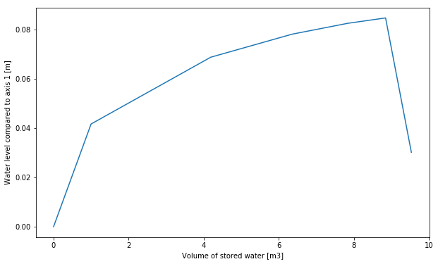
Result of the ponding analysis.
The analysis results in the diagram above. We can see the maximum water level capacity of this structure in one diagram! At a stored water volume of 9.5 m3 the maximum water level is reached. When the roof stores more water it starts to accumulate eventually resulting in failure.
If we want to examine the results visually at the moment of accumulating water we can call for a plot:
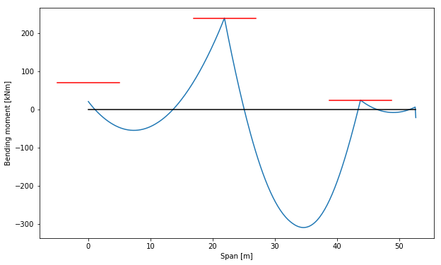
ss.show_bending_moment(verbosity=1)
Bending moment when the roof starts accumulating.
This is gives us a proper indication of the way the bending moments are divided across the structure. We can clearly see that the node on axis 3 exceeds its yielding capacity, as there is almost none hogging bending moment visible. However before stating that such an analysis is correct, we should do some checks.
## Sanity check As a validation we'll only check the occurring bending moments and the capacity they should have.
In the diagram below we can see that both axis 2 and axis 3 have yielding nodes exactly on the maximum moment we assigned to those nodes. The bending moment at axis 1 isn’t that large due to the relatively low rotational spring of 9.000 kNm/rad. The bending moments don’t seem to exceed our given boundaries, so we can conclude that the non linear behavior is computed as expected.
plt.plot(ss.nodes_range('x')[:-2], [el.bending_moment[0] for el in list(ss.element_map.values())[:-1]])
a = 0
plt.plot([0, p6.x], [a, a], color="black")

c = "red"
a = 240
plt.plot([p3.x - 5, p3.x + 5], [a, a], color=c)
a = 25
plt.plot([p5.x - 5, p5.x + 5], [a, a], color=c)
a = 70
plt.plot([p1.x - 5, p1.x + 5], [a, a], color=c)

plt.ylabel("Bending moment [kNm]")
plt.xlabel("Span [m]")
plt.show()
Bending moment when the roof starts accumulating.
Accumulating span
If we substract the deflection from the structures height, we’ll see the final state of the structure (during accumulating of the water). The figure below shows that the span between axis 2 and axis 3 is accumulating water. These are just fun plots, and if you save these every iteration it can give a nice animation of how the structure is failing.
plt.plot(ss.nodes_range('x')[:-2], ss.nodes_range('y')[:-2])
plt.plot(ss.nodes_range('x')[:-2], [a + b for a, b in zip(ss.nodes_range('y')[:-2], ss.get_node_result_range("uy")[:-2])])

plt.ylabel("Height level roof when accumulating [m]")
plt.xlabel("Span [m]")
plt.show()
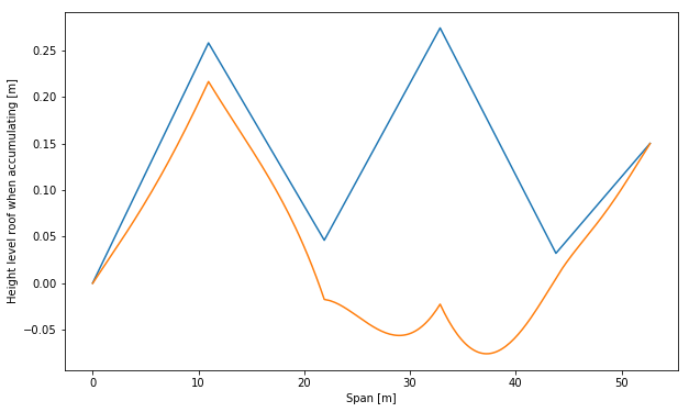
Final state of the structure at the moment of accumulating
Conclusion
In this post we’ve done a water accumulation analysis in anaStruct. I’ve done the analysis for this post in a notebook, which can be downloaded here.
We’ve setup a calculation that is comparable with ‘real’ world engineering problems. We’ve computed the maximum water storage capacity of this structure. The fact that we can do such an analysis in just a few minutes, makes it possible to compute more combinations of stiffness properties and bending moment capacities and gain more insights in valid ways to make it more endurable to ponding.
Water accumulation problems are complex problems that require nummerical approaches in most cases. The fact that you need to do this analysis with springs, non-linear nodes, iteratively, non linear and maybe even geometrical non linear, makes it a problem that is not easily solved and makes you most of the times dependent of expensive software.
And now we can do it in Python :)