Last [Algorithm Breakdown](https://www.ritchievink.com/blog/2018/09/26/algorithm-breakdown-ar-ma-and-arima-models/) we build an ARIMA model from scratch and discussed the use cases of that kind of models. ARIMA models are great when you have got stationary data and when you want to predict a few time steps into the future. A lot of business data, being generated by human processes, have got weekly and yearly seasonalities (we for instance, seem work to less in weekends and holidays) and show peaks at certain events. This kind of data is measured a lot and there is time series expertise needed to model this correctly. Facebook has released an open source tool, Prophet, for analyzing this type of business data. Prophet is able to fit a robust model and makes advanced time series analysis more available for laymen.
This post we break down the components of Prophet and implement it in PyMC3.
Generalized Additive Models
Prophet is based on Generalized Additive Models, which is actually nothing more than a fancy name for the summation of the outputs of different models. In Prophets case, it is the summation of a trend $g(t)$, a seasonal series $s(t)$, and a holiday effect (special events) $h(t)$.
$$ y(t) = g(t) + s(t) + h(t) + \epsilon_t \tag{1}$$
$y(t)$ is the time series data we observe at time $t$, and $\epsilon$ is some stochastic process we cannot explain.
With a probabilistic framework such as Stan or Pymc3, we can define priors on the parameters of terms $g(t)$, $s(t)$, and $h(t)$ and then sample the posterior distribution to find the maximum likelihood of $y(t)$ (observed data). Facebook has implemented this model in probabilistic framework Stan. We are going to implement it in Pymc3. In this post, we will only focus on the terms $g(t)$ and $s(t)$ as that covers the gist of the problem. Implementing $h(t)$ is an easy extension which I leave for the enthusiastic readers.
Linear Trend with Changepoints
We will model a piece-wise constant growth described by
$$ g(t) = (k + a(t)^T \delta)t + (m + a(t)^T \gamma) \tag{2}$$
where $k$ is the growth rate, $m$ is the offset parameter, $\delta$ is a vector with growth rate adjustments, and $\gamma_j$ is set to $-s_j \delta_j$, where $s_j$ is a changepoint in time.
This growth model consists of a base trend $k$ and preset changepoints at which the growth rate can be adjusted by $s_j$. Those preset changepoints are defined in a vector with $S$ changepoints at times $s_j$, $j = 1, …, S$. At each unique changepoint $s_j$, the growth rate is adjusted by $\delta_j$. We can define all growth rate adjustments by the vector $\delta \in \mathbb{R}^S$
The growth rate is adjusted every time step that $t$ surpasses a changepoints $s_j$, the growth rate becomes the base rate plus the sum of all adjustments up to that point
$$ k + \sum_{j: t > s_j} \delta_j \tag{3}$$
Eq (3) can be vectorized by defining $a(t) \in {0, 1}^S$ such that
a(t)=
\begin{cases} 1, & \text{if } t\geq s_j, \ 0, & \text{otherwise} \end{cases}
\tag{4} $$
By taking the dot product, all the changepoints $s_j > t$ cancel out. The growth rate at time $t$ is then
$$ k + a(t)^T \delta \tag{5} $$
We can actually rewrite the whole function for all time values $t$ by defining a matrix $A$.
As an example, let $S$ be the changepoints $2, 5, 8$, and time steps $t = 1, 2, \dots, 10$
A = \begin{bmatrix} t_{1} \geq s_1 & t_{1} \geq s_2 & \dots & t_{1} \geq s_n \ t_{2} \geq s_1 & t_{2} \geq s_2 & \dots & t_{2} \geq s_n \ \vdots & \vdots & \ddots & \vdots \ t_{k} \geq s1 & t_{k} \geq s_2 & \dots & t_{k} \geq s_n \end{bmatrix}
=
\begin{bmatrix} 1 \geq 2 & 1 \geq 5 & 1 \geq 8 \ 2 \geq 2 & 2 \geq 5 & 2 \geq 8 \ \vdots & \vdots & \vdots \ 10 \geq 2 & 10 \geq 5 & 10 \geq 8 \end{bmatrix}
=
\begin{bmatrix} 0 & 0 & 0 \ 1 & 0 & 0 \ \vdots & \vdots & \vdots \ 1 & 1 & 1 \end{bmatrix}
$$
Eq. (2) then becomes
$$ \vec{g} = (k + A \vec{\delta}) \odot \vec{t} + (m + A \vec{\gamma}) \tag{6}$$
Let’s get a feel for this formula by plotting different components.
# one shot import all we need for this post
import numpy as np
import pymc3 as pm
import matplotlib.pyplot as plt
from scipy import stats
import pandas as pd
import theano
import theano.tensor as tt
from fbprophet import Prophet

np.random.seed(25)
n_changepoints = 10
t = np.arange(1000)
s = np.sort(np.random.choice(t, n_changepoints, replace=False))

A = (t[:, None] > s) * 1
delta = np.random.normal(size=n_changepoints)
k = 1
m = 5

growth = (k + A @ delta) * t
gamma = -s * delta
offset = m + A @ gamma
trend = growth + offset

plt.figure(figsize=(16, 3 * 3))
n = 310
i = 0
for t, f in zip(['Linear Trend with Changepoints', 'Growth rate', 'Growth offset'],
                [trend, growth, offset]):
    i += 1
    plt.subplot(n + i)
    plt.title(t)
    plt.yticks([])
    plt.vlines(s, min(f), max(f), lw=0.8, linestyles='--')
    plt.plot(f)
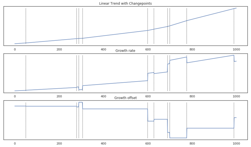
Components of the piecewise linear trend function.
Above we see the result of the piecewise linear trend with changepoints. The changepoints are shown by vertical dashed lines. The first plot shows the result of the whole trend function as a reasonable continuous trend. The middle plot shows the growth rate $ k + \sum_{j: t > s_j} \delta_j $ at time $t$. The last plot shows the offset at time $t$. These are just horizontal plateaus that adjust the growth rate’s height in order to generate a continuous plot.
Trend model
Let’s implement this first part of the model. For some vague reason, the PyMC3’s NUTS sampler doesn’t work if I use Theano’s (the framework in which PyMC3 is implemented) dot product function tt.dot. Therefore we quickly implement our own.
def det_dot(a, b):
    """
    The theano dot product and NUTS sampler don't work with large matrices?

    :param a: (np matrix)
    :param b: (theano vector)
    """
    return (a * b[None, :]).sum(axis=-1)
Data
Let’s also load and prepare some data. We are going to use the same dataset as Facebook does in their Quick Start tutorial of Prophet. The csv file can be downloaded here.
df = pd.read_csv('peyton_manning.csv')
# Make sure we work with datetime types
df['ds'] = pd.to_datetime(df['ds'])
# Scale the data
df['y_scaled'] = df['y'] / df['y'].max()
df['t'] = (df['ds'] - df['ds'].min()) / (df['ds'].max() - df['ds'].min())
df.plot(x='ds', y='y', figsize=(16, 6), title="Wikipedia pageviews for 'Peyton Manning'")

Daily pageviews of Peyton Manning's Wikipedia page.
Below we define the PyMC3 implementation of the piecewise linear trend model. The standard model is defined by
$$ k \sim N(0, 5) $$ $$ \delta \sim Laplace(0, 0.05) $$ $$ m \sim N(0, 5) $$ $$ g|k, \delta, m = (k + A \delta) \odot t + (m + A (-s \odot \delta)) $$ $$ \sigma \sim N(0, 0.5) $$ $$ y| g, \sigma \sim N(g, \sigma) $$
In Python/ PyMC3 this translates to
def trend_model(m, t, n_changepoints=25, changepoints_prior_scale=0.05,
                growth_prior_scale=5, changepoint_range=0.8):
    """
    The piecewise linear trend with changepoint implementation in PyMC3.
    :param m: (pm.Model)
    :param t: (np.array) MinMax scaled time.
    :param n_changepoints: (int) The number of changepoints to model.
    :param changepoint_prior_scale: (flt/ None) The scale of the Laplace prior on the delta vector.
                                    If None, a hierarchical prior is set.
    :param growth_prior_scale: (flt) The standard deviation of the prior on the growth.
    :param changepoint_range: (flt) Proportion of history in which trend changepoints will be estimated.
    :return g, A, s: (tt.vector, np.array, tt.vector)
    """
    s = np.linspace(0, changepoint_range * np.max(t), n_changepoints + 1)[1:]

    # * 1 casts the boolean to integers
    A = (t[:, None] > s) * 1

    with m:
        # initial growth
        k = pm.Normal('k', 0 , growth_prior_scale)

        if changepoints_prior_scale is None:
            changepoints_prior_scale = pm.Exponential('tau', 1.5)

        # rate of change
        delta = pm.Laplace('delta', 0, changepoints_prior_scale, shape=n_changepoints)
        # offset
        m = pm.Normal('m', 0, 5)
        gamma = -s * delta

        g = (k + det_dot(A, delta)) * t + (m + det_dot(A, gamma))
    return g, A, s

# Generate a PyMC3 Model context
m = pm.Model()

with m:
    y, A, s = trend_model(m, df['t'])

    sigma = pm.HalfCauchy('sigma', 0.5, testval=1)
    pm.Normal('obs',
                 mu=y,
                 sd=sigma,
                 observed=df['y_scaled'])
Sanity check
Before we run the model, let’s define a small utility function. This function samples from the prior distribution of the model we defined and plots the expected value given the prior, i.e. the mean, and the standard deviation of the sampled values.
def sanity_check(m, df):
    """
    :param m: (pm.Model)
    :param df: (pd.DataFrame)
    """
    # Sample from the prior and check of the model is well defined.
    y = pm.sample_prior_predictive(model=m, vars=['obs'])['obs']
    plt.figure(figsize=(16, 6))
    plt.plot(y.mean(0), label='mean prior')
    plt.fill_between(np.arange(y.shape[1]), -y.std(0), y.std(0), alpha=0.25, label='standard deviation')
    plt.plot(df['y_scaled'], label='true value')
    plt.legend()

# And run the sanity check
sanity_check(m, df)
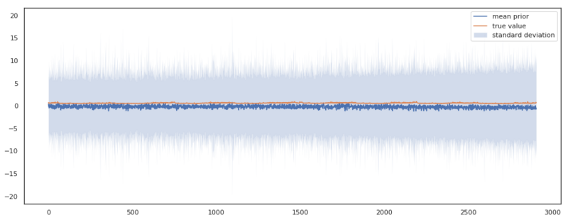
Outputs sampled from the prior distribution of the trend model.
Above we see the results of the sanity check. The expected output of the model shows a constant expected value of 0 and a reasonable constant standard deviation of $\pm$ 10. We can see that there is an offset between the true value and the mean prior. By eyeballing it, I would say it is an offset of about 1, which is well covered for in our prior of the offset $m \sim N(0, 5)$, as it assigns plenty probability to $m = 5$. This kind of plots really helps you in parameterizing your model, and reason about the sanity of your results. If we, for instance, hadn’t scaled the time values $t$, the output would have looked like this. Giving a strong indication that our model is not well defined.
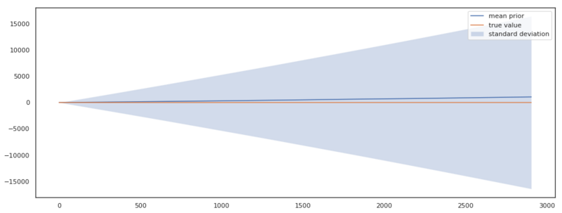
Outputs sampled from the prior distribution of the trend model when the input variables $t$ are not scaled.
Inference
Now we are going infer the parameters of our model by doing a Maximum A Posteriori (MAP) estimation. This is an estimation of the mode of the posterior distribution. This estimation is also just a point estimate distribution, meaning that we will not have any information about the posteriors shape. As the dimensionality of a problem increases, it gets more and more unlikely that the mode equals the region of highest probability as the mass of the distribution can be situated on a whole different region. The example below shows such a case with a bimodal distribution.
x = np.linspace(-10, 10, 1000)
pdf = stats.norm.pdf(x, -2, 1) + stats.norm.pdf(x, 5, 0.05) * 0.06
mode = pdf.max()
mean = pdf.mean()

# find the mean of the integrated probablity density function
idx_mean = np.argmin(np.abs(np.cumsum(pdf) - np.cumsum(pdf).mean()))
idx_mode = pdf.argmax()
plt.figure(figsize=(16, 6))
plt.plot(x, pdf)
plt.vlines([x[idx_mean], x[idx_mode]], 0, mode, lw=0.8, linestyles='--')
plt.annotate('mean', (x[idx_mean] + 0.2, mode * 0.9))
plt.annotate('mode', (x[idx_mode] + 0.2, mode * 0.9))
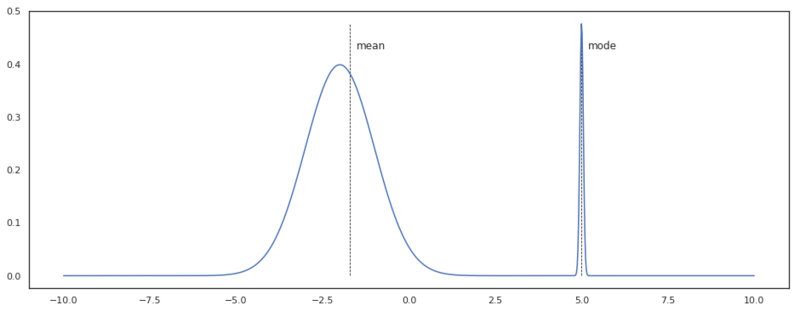
Bimodal distribution, where the mode is in a region with a lower probability mass than the mean.
Nonetheless, we are going to estimate the parameters of our model with MAP. Later in this post, we will approximate the posterior distribution by sampling with Markov Chain Monte Carlo (MCMC) and look at the benefits this yields.
# Find a point estimate of the models parameters
with m:
    aprox = pm.find_MAP()

# Determine g, based on the parameters
def det_trend(k, m, delta, t, s, A):
    return (k + np.dot(A, delta)) * t + (m + np.dot(A, (-s * delta)))

# run function and rescale to original scale
g = det_trend(aprox['k'], aprox['m'], aprox['delta'], df['t'], s, A) * df['y'].max()

plt.figure(figsize=(16, 6))
plt.title('$g(t)$')
plt.plot(g)
plt.scatter(np.arange(df.shape[0]), df.y, s=0.5, color='black')
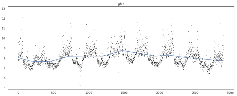
Result of piecewise linear trend with changepoints.
Above we see the result of our parameter estimation, which looks pretty reasonable. We see that the model has remained quite a linear trend. This is due to the prior we have set on the changepoint_prior, $\tau = 0.05$. If we would increase this value, the model would have more flexibility and be able to follow the variance better, but as a result, have a higher probability of overfitting to the data.
Seasonality
Of course, we cannot forecast business time series, without modelling seasonalities. Prophet models seasonalities for daily, weekly, monthly and yearly patterns, all based on Fourier series. In this post, we will only focus on weekly and yearly seasonality, but adding more will be easy!
A Fourier series is described by
$$ s(t) = \sum_{n=1}^N(a_n cos(\frac{2\pi nt}{P}) + b_n sin(\frac{2 \pi nt}{P})) \tag{7}$$
Here $P$ is the period we want to model as seasonal effect. For yearly data $P = 365.25$, and for weekly data $P = 7$. $N$ is the order of the Fourier series. Prophet uses $N = 10$ for yearly data and $N = 3$ for weekly data. We can generate a matrix $X(t)$ containing parts of eq. (7) for each value of $t$. With weekly data, this will result in
$$ X(t) = [cos( \frac{2\pi 1t}{7}), …, sin(\frac{2\pi 3t}{7})] \tag{8}$$
Our model should then have parameters $\beta \in \mathbb{R}^{2N}$, $\beta = a_1, b_1, …, a_n, b_n$.
The seasonal component is then
$$ s(t) = X(t) \beta \tag{9}$$
Let’s define the matrix $X(t)$ in Python and test the result with a randomly initialized vector $\beta$.
np.random.seed(6)
def fourier_series(t, p=365.25, n=10):
    # 2 pi n / p
    x = 2 * np.pi * np.arange(1, n + 1) / p
    # 2 pi n / p * t
    x = x * t[:, None]
    x = np.concatenate((np.cos(x), np.sin(x)), axis=1)
    return x

n = 4
t = np.arange(1000)
beta = np.random.normal(size=2 * n)
plt.figure(figsize=(16, 6))
plt.plot(fourier_series(t, 365.25, n) @ beta)
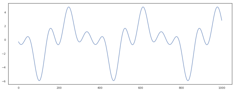
Example of a Fourier series with order 4 and a period of 365.25.
Complete model
Now we’ve set up all we need for our complete model. We mentioned earlier that Prophet, estimates a maximum point estimate of the posterior distribution. We are going to sample in order to estimate the posterior. By sampling, we are will not find values for our parameters, but find whole distributions! This is great! We will have a lot of information about the uncertainty of our predictions by analyzing the posterior distributions, or by just sampling the posterior! I think this is very cool, and see this as one of the best properties of Bayesian modeling.
Different from the base model, we will now set a hierarchical prior on the changepoint_prior_scale $\tau$. In the base model, this was set to $\tau = 0.05$. This base prior is pretty restrictive, giving the model not too much flexibility to fit the data. Because we will not restrict the model as much, we probably have a trend that is more able to fit the data.
The complete model is now defined as
$$ k \sim N(0, 5) $$ $$ \tau \sim Exponential(1.5) $$ $$ \delta| \tau \sim Laplace(0, \tau) $$ $$ m \sim N(0, 5) $$ $$ g|k, \delta, m, \tau = (k + A \delta) \odot t + (m + A (-s \odot \delta)) $$ $$ \beta \sim N(0, 10) $$ $$ s| \beta = X(t) \beta $$ $$ \sigma \sim HalfCauchy(0, 0.5) $$ $$ y| g, \sigma, s \sim N(g + s, \sigma) $$
Below we build the model defined above. First, we define a function seasonality_model which initiates the priors $\beta$ for seasonality regression. Note that we MinMax scale the period of the Fourier series, as $t$ is also MinMax scaled. The prior output is defined by
$$ y(t) = g(t) + s(t)_{weekly} + s(t)_{yearly} + \epsilon_t \tag{10}$$
def seasonality_model(m, df, period='yearly', seasonality_prior_scale=10):

    if period == 'yearly':
        n = 10
        # rescale the period, as t is also scaled
        p = 365.25 / (df['ds'].max() - df['ds'].min()).days
    else:  # weekly
        n = 3
        # rescale the period, as t is also scaled
        p = 7 / (df['ds'].max() - df['ds'].min()).days
    x = fourier_series(df['t'], p, n)
    with m:
        beta = pm.Normal(f'beta_{period}', mu=0, sd=seasonality_prior_scale, shape=2 * n)
    return x, beta

m = pm.Model()

with m:
    # changepoints_prior_scale is None, so the exponential distribution
    # will be used as prior on \tau.
    y, A, s = trend_model(m, df['t'], changepoints_prior_scale=None)
    x_yearly, beta_yearly = seasonality_model(m, df, 'yearly')
    x_weekly, beta_weekly = seasonality_model(m, df, 'weekly')

    y += det_dot(x_yearly, beta_yearly) + det_dot(x_weekly, beta_weekly)

    sigma = pm.HalfCauchy('sigma', 0.5, testval=1)
    obs = pm.Normal('obs',
                 mu=y,
                 sd=sigma,
                 observed=df['y_scaled'])
And we start MCMC sampling by
with m:
    trace = pm.sample(500)
pm.traceplot(trace)
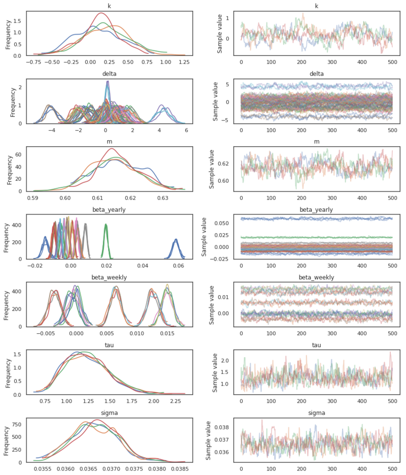
Posterior parameter distribution.
Above we see the result of our MCMC sampling. We have found an estimate of the posterior distribution of our parameters. Now that we have got this, we can take a look at how the model has fit the data. Below we are computing the trend and the seasonalities for all the drawn samples. This will result in a matrix of shape $T \times S$, with $T$ being the number of data points and $S$ the number of drawn samples. With this matrix, we can finally compute the credible intervals of our fit. Below is the plot shown with credible intervals of 95%.
def det_seasonality_posterior(beta, x):
    return np.dot(x, beta.T)

p = 0.025
# vector distributions
beta_yearly = trace['beta_yearly']
beta_weekly = trace['beta_weekly']
delta = trace['delta']

# scalar distributions
k = trace['k']
m = trace['m']

# determine the posterior by evaulating all the values in the trace.
trend_posterior = ((k + np.dot(A, delta.T)) * df['t'][:, None] + m + np.dot(A, (-s * delta).T)) * df['y'].max()

yearly_posterior = det_seasonality_posterior(beta_yearly, x_yearly) * df['y'].max()
weekly_posterior = det_seasonality_posterior(beta_weekly, x_weekly) * df['y'].max()

date = df['ds'].dt.to_pydatetime()
sunday = np.argmax(df['ds'].dt.dayofweek)
weekdays = ['sunday', 'monday', 'tuesday', 'wednesday', 'thursday', 'friday', 'saturday']
idx_year = np.argmax(df['ds'].dt.dayofyear)

plt.figure(figsize=(16, 3*6))
b = 411
plt.subplot(b)
plt.title('total')
plt.plot(date,
         (trend_posterior + yearly_posterior + weekly_posterior).mean(1), lw=0.5)
plt.scatter(date, df['y'], s=0.5, color='black')

plt.subplot(b + 1)
plt.title('trend')
plt.plot(date, trend_posterior.mean(1))
quant = np.quantile(trend_posterior, [p, 1 - p], axis=1)
plt.fill_between(date, quant[0, :], quant[1, :], alpha=0.25)

plt.subplot(b + 2)
plt.title('yearly')
plt.plot(date[idx_year: idx_year + 365], yearly_posterior.mean(1)[idx_year: idx_year + 365])
quant = np.quantile(yearly_posterior, [p, 1 - p], axis=1)
plt.fill_between(date[idx_year: idx_year + 365],
                 quant[0, idx_year: idx_year + 365], quant[1, idx_year: idx_year + 365], alpha=0.25)

plt.subplot(b + 3)
plt.title('weekly')
plt.plot(weekdays, weekly_posterior.mean(1)[sunday: sunday + 7])
quant = np.quantile(weekly_posterior, [p, 1 - p], axis=1)
plt.fill_between(weekdays, quant[0, sunday: sunday + 7],
                 quant[1, sunday: sunday + 7], alpha=0.25)
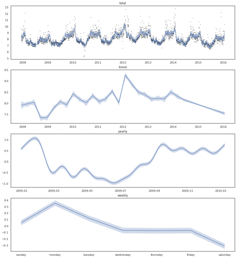
Fitted model with 95% credible intervals.
Trend forecasts and uncertainty
The uncertainty of the predictions you make in Prophet is determined by the number of changepoints that are allowed, whilst fitting the training data and the flexibility of the changepoint adjustments $\delta$. Intuitively, it says that if we have seen a lot of change in the time history, we can expect a lot of change in the future.
The uncertainty is modeled by sampling changepoints and change adjustments following the rule
\forall j > T,
\begin{cases} \delta_j = 0 \quad w.p. \frac{T - S}{T} \ \delta_j \sim Laplace(0, \lambda) \quad w.p. \frac{S}{T} \end{cases}
\tag{11} $$
where $T$ is the complete history, and $S$ are the number of changepoints fitted in the training data. For all time steps larger than $T$ there is a probability of occurring a new changepoint $\delta_j$, which is sampled from a Laplace distribution. The scale $\lambda$ of the Laplace distribution is determined by one of the following.
- The mean of the posterior of the hyperprior $\tau$
- If the hyperprior is not set, $\lambda = \frac{1}{S} \sum_{j=1}^S |\delta_j|$.
Below we implement a trend forecast and the uncertainty as defined above. We continue with the trace of our earlier sampled model. Because we have defined a hyperprior $\tau$ we can use that as scale parameter $\lambda$ for the Laplace distribution.
n_samples = 1000
days = 150
history_points = df.shape[0]
probability_changepoint = n_changepoints / history_points

future = pd.DataFrame({'ds': pd.date_range(df['ds'].min(),
                                           df['ds'].max() + pd.Timedelta(days, 'D'),
                        df.shape[0] + days)})
future['t'] = (future['ds'] - df['ds'].min()) / (df['ds'].max() - df['ds'].min())

# vector distributions
beta_yearly = trace['beta_yearly'].mean(0)
beta_weekly = trace['beta_weekly'].mean(0)
delta = trace['delta'].mean(0)

# scalar distributions
k = trace['k'].mean()
m = trace['m'].mean()

trend_forecast = []
lambda_ = trace['tau'].mean()

for n in range(n_samples):
    new_changepoints = future['t'][future['t'] > 1].values
    sample = np.random.random(new_changepoints.shape)
    new_changepoints = new_changepoints[sample <= probability_changepoint]
    new_delta = np.r_[delta,
                      stats.laplace(0, lambda_).rvs(new_changepoints.shape[0])]
    new_s = np.r_[s, new_changepoints]
    new_A = (future['t'][:, None] > new_s) * 1

    trend_forecast.append(((k + np.dot(new_A, new_delta)) * future['t']  + (m + np.dot(new_A, (-new_s * new_delta)))) * df['y'].max())

trend_forecast = np.array(trend_forecast)

date = future['ds'].dt.to_pydatetime()
plt.figure(figsize=(16, 4))
plt.title('Trend forecasts uncertainty')
plt.plot(date, trend_forecast.mean(0))
quant = np.quantile(trend_forecast, [0.025, 0.975], axis=0)
plt.fill_between(date, quant[0, :], quant[1, :], alpha=0.25)
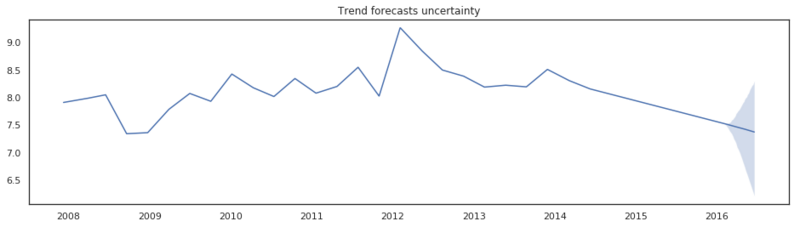
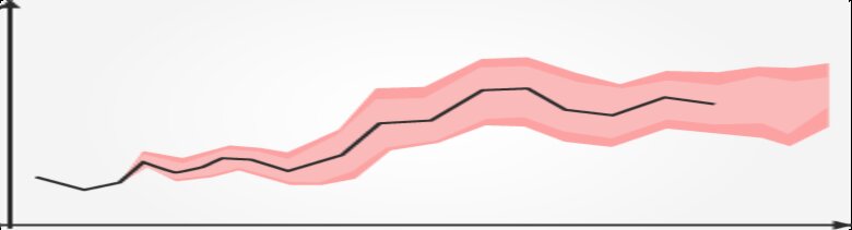
Trend forecast with 95% credible intervals.
Above we see the result of 1000 samples. Due to the flexibility of the hyperprior $\tau$ the model was able to fit the data very well. However by doing so the variance of the changepoints adjustments $\delta$ is quite high, resulting in wide uncertainty bands.
Final words
The last model we set a hyperprior on $\tau$. If we don’t set this hyperprior and instead and use the changepoint_scale_prior = 0.05 we get exactly the same results as Facebook Prophet gets in their Quick Start tutorial. The Prophet implementation comes with more features than we discussed in this post. Their implementation also has an option to model recurring events, (they call them holidays). With the base of this model ready, it is fairly easy to add another linear model that is dependent on other
predictors like the weather. Facebook writes in the introduction of their paper, that Prophet is a good plug and play library for business analysts to do time series analysis. Besides that, it is a very good Bayesian base model to further implement while modeling time series.
Want to read more Algorithm Breakdowns?