This post describes the implementation of a linear support vector machine classifier (SVM) in Scala. Scala is a functional programming language that supports functional programming to a far extend. Because I am exploring Scala at the moment and I like the challenge of functional programming, the SVM will be implemented in a functional manner. We are going to test the SVM on two classes from the Iris dataset.
Linear Support Vector Machine intuition
Support Vector Machines are binary classifiers. They label different classes by seperating them with a linear hyperplane.
A hyperplane sounds like an attack straight from a Dragonball Z episode, but I can assure you it is less impressive. If our feature space (The amount of columns in our dataset) is 1 dimensional, a hyperplane would be a point. Is the feature space 2 dimensional, than the hyperplane is a line. In a 3 dimensional feature space the hyperplane is a plane. Formally a hyperplane is a geometric space one dimension less than the feature space. Below are some hyperplanes shown in the few dimensions I am comfortable at.
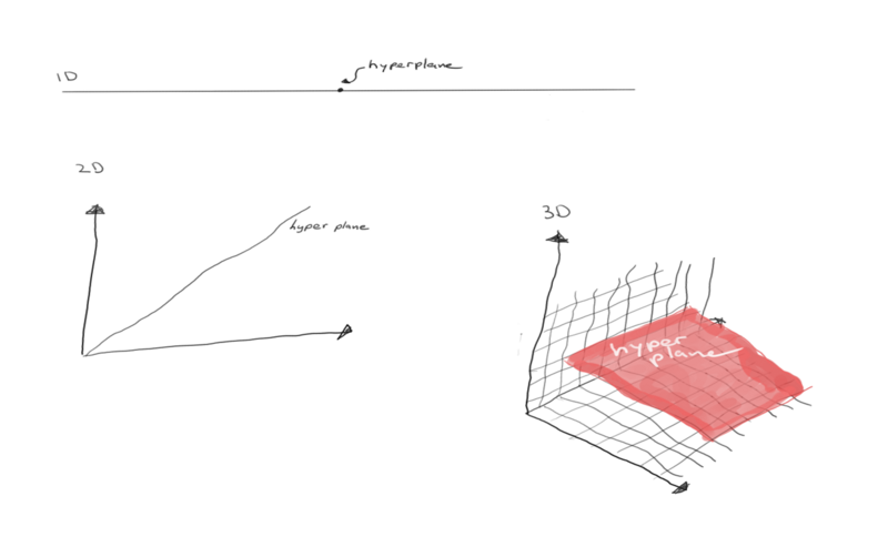
Hyperplanes at different dimensions.
To keep things simple we are going to look at only two dimensions and two classes. We can imagine having two classes, the red pills and the green pills, as shown in the image below. A support vector machine tries to draw a hyperplane that splits these two classes. However in this case the classes are linearly seperable by an infinite number of lines. In the figure this infinite number of lines is illustrated with two lines. As this is the first time I borrowed the drawing tablet from my girlfriend and thus am really slooow in making this sketches I stopped at two.
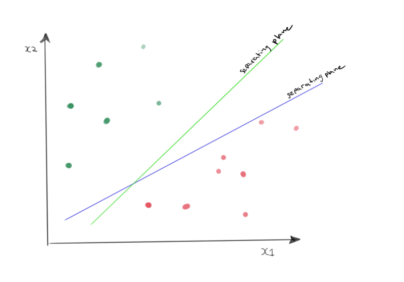
Optimal hyperplane?
Although not close to infinite, those two lines do illustrate the problem. The SVM must find the optimal hyperplane that splits the observed data points best. Therefore there needs to be a definition of optimal seperating hyperplane.
The optimal hyperplane is defined by the plane that maximizes the perpendicular distance between the hyperplane and the closest samples. This perpendicular distance can be spanned with support vectors.
Below is an example of a suboptimal and an optimal separating hyperplane. The optimal hyperplane maximizes the support vectors lenth.
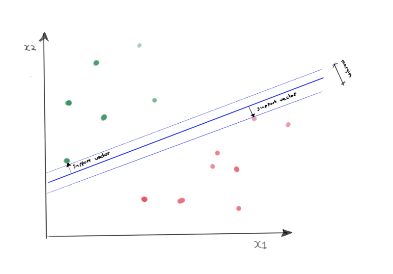
Suboptimal separating hyperplane.
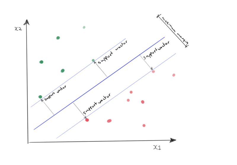
Optimal separating hyperplane.
Linear Support Vector Machine model
Now we’ve defined what a support vector machine is, let’s take a look at the model definition. As noted at the beginning of this post, SVM’s are binary models. This means we can only label two classes. Those classes need to be labeled as either +1 or -1. The linear support vector machine model is relatively simple. The hyperplane must fulfil the following equation:
Where:
- \( \vec{x}: \) is the feature vector
- \( \vec{w}: \) is the models weights vector
- \( b: \) is the bias value
The outer hyperplanes of the margins. The ones that are spanned by the support vectors should fulfil the following properties:
For class y = -1:
For class y = 1:
The absolute values for samples that are situated outside this margin will have values > 1. The model classifies an input by looking at the sign of the result:
Classification of a new data point:
Below you’ll see the support vector machine model in relation to the dataset. You’ll also see that I am getting slightly better at handling a drawing tablet!
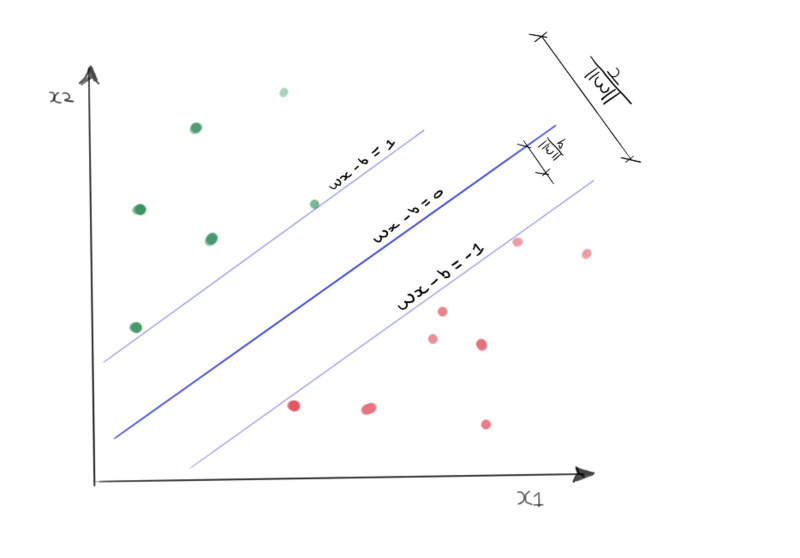
Support vector machine model.
Optimization
The variables of the model \( \vec{x} \) and \( b \) are still unknown. We can find them using gradient descent. Therefore we need a loss function.
linearly seperable classes
For a model that is trained on data that is linearly seperable (like the data in my beautiful sketches ♥) the following constraint holds for all data points \( i \).
Given the label \( y_i \):
\( \vec{x} \cdot \vec{w} - b \geq 1 \) for every \( y_i = 1 \)
\( \vec{x} \cdot \vec{w} - b \leq -1 \) for every \( y_i = -1 \)
This results in the following restriction:
The loss function \( J \) we can minimize is the ‘Hinge loss’ function:
Not linearly seperable classes
When data is not linearly seperable there cannot be a ‘hard margin’ between the data samples and the margin that is spanned by the support vectors. A SVM trained on not linearly seperated data is called a ‘soft margin’ SVM. In such a case a regularization term \( \lambda ||\vec{w}||^2 \) is added.
The loss function then becomes:
Where \( \lambda \) is a regularization parameter that controls the trade off between a hard margin and soft margine. In other words, a trade off between following noise in the data or generalizing (with a chance of underfitting).
Partial derivatives
As we will update the weights of the model using gradient descent we need the determine the partial derivates of the loss function with respect to the weights.
First part of the loss function
To make the formulation a little bit easier and more like the way we are going to implement the bias term in code. We will concatenate the bias term \( b \) to the weight vector \( \vec{w} \). The first part of loss function can then be written as:
If we look at the loss function we can see that when the model classifies \( y_i \) correctly the result will be \( \geq 1 \). The second parameter of the max function will in that case be 0 or negative, leading to a maximum loss of 0. This leads to our first partial derivative:
CASE model classifies \( y_i \) correct:
When the classification is incorrect, the loss is:
CASE model classifies \( y_i \) incorrect:
And finaly we’ve got the partial derivative of the regularization term:
Scala implementation
Now we have the dealt with the technicallities we can write the code for our support vector machine. The complete code and the dataset is hosted on github.
Data
The ./res folder holds a csv file with the iris dataset.
First we implement a method to load the data. Because the SVM model is binary we discard the ‘virginica’ flower
type DataFrame[A] = Vector[Vector[A]]

object readCSV {
  /**
    * Reads the iris dataset and return the 'setosa' and 'versicolor' class and takes the first two feature columns.
    *
    * @param path Path of the iris.csv file
    * @return a dataframe containing the features and the labels.
    */
  def apply(path: String): (DataFrame[Double], Vector[Int]) = {
    val bufferedSource = scala.io.Source.fromFile(path)

    // rename the setosa and versicolor class to -1 and 1
    def flowerClass(v: String): Double = v.trim() match {
      case "setosa" => -1
      case "versicolor" => 1
      case "virginica" => 10
      case x => x.toDouble
    }

    // read lines
    val lines = bufferedSource.getLines.toVector.tail

    // split lines and map the flowerClass function discarding the virginica flower.
    val rows = lines.map(_.split(",").map(flowerClass)).filter(i => i.last < 2)
    val labels = rows.map(_.last.toInt)
    val data = rows.map(_.init)
    bufferedSource.close()

    (data.map(i => Vector(i(0), i(1))), labels)
  }
}
The iris dataset has a feature space of 4 dimensions. Because we want to be able to plot separating hyperplace easily we are going to train the SVM on only the first two features. If we plot those we’ll see the following figure.
import breeze.plot._

val f = Figure()
val p = f.subplot(0)
p.title = "'setosa' and 'versicolor'"
p.xlabel = "x1"
p.ylabel = "x2"

// filter the feature values by the classes 1 and -1
val x1 = (df, labels).zipped.filter((_, b) => b == -1)._1
val x2 = (df, labels).zipped.filter((_, b) => b == 1)._1

p += plot(x1.map(_(0)), x1.map(_(1)), '.', "b")
p += plot(x2.map(_(0)), x2.map(_(1)), '.', "r")
f.saveas("fig.png")
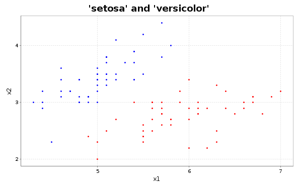
The setosa and versicolor flower labels
We can tell from the figure that the two classes are clustered nicely. They seem completely linearly seperable. The SVM we are building should be able to find an optimal hard margin hyperplane based on this figure.
SVM Class
For the SVM class we start with a constructor that takes as arguments the data x, the labels, the learning rate eta and the number of training epochs. As we only regard the first two feature dimensions we create a new DataFrame df containing the first two feature rows and a bias term that equals 1.
Next we initialize the weights vector w with zeros.
Constructor
class Svm(x: DataFrame[Double], labels: Vector[Int], eta: Double=1, epochs: Int=10000) {

  // add a bias term to the data
  def prepare(x: DataFrame[Double]): DataFrame[Double] = x.map(_ :+ 1.0)

  // Prepared data
  val df: DataFrame[Double] = prepare(x)

  // weights initialization
  var w :Vector[Double] = (for (_ <- 1 to df(0).length) yield 0.0).toVector

}
As noted before, the classifcation of the model was described by:
So we can add a classification method. But first we need a functions that returns the dot product of two vectors.
Dot product function
object dotProduct {
  def apply(x: Vector[Double], w: Vector[Double]): Double = {
        (x, w).zipped.map((a, b) => a * b).sum
    }
}
The classification method than becomes:
Classifier
def classification(x: Vector[Vector[Double]], w: Vector[Double] = w): Vector[Int] = {
    x.map(dotProduct(_, w).signum)
}
Finally we can implement the training method. This method will update the weights by applying eq 1. and eq. 2. The fit method implements the training of the SVM model. It returns Unit, because it changes the state of the weights.
The functions gradient and regularizationGradient are eq 1. and eq. 2 respectively. The function misClassification is a helper function used in the pattern matching guards of the trainOneEpoch function.
This trainOneEpoch is tail recursive and iterates over all the data samples. If a classification is correct it will update the weights according to regularizationGradient, if the classification is incorrect, the weights are updated with gradient.
The last function is trainEpochs which is also tail recursive and will iterate until epochCount == 0.
The call order of the functions is trainEpochs → trainOneEpoch → {gradient, regularizationGradient, misClassification}. Note that both gradient methods have a value of 1 / epoch wich are a decreasing learning rate, making the learning more stable.
Training method
  def fit(): Unit = {
    // Will only be called if classification is wrong.
    def gradient(w: Vector[Double], data: Vector[Double], label: Int, epoch: Int): Vector[Double] = {
      (w, data).zipped.map((w, d) => w + eta * ((d * label) + (-2 * (1 / epoch) * w)))
    }

    // Misclassification treshold.
    def misClassification(x: Vector[Double], w: Vector[Double], label: Int): Boolean = {
      dotProduct(x, w) * label < 1
    }

    def regularizationGradient(w: Vector[Double], label: Int, epoch: Int): Vector[Double] = {
      w.map(i => i + eta * (-2  * (1 / epoch) * i))
    }

    def trainOneEpoch(w: Vector[Double], x: DataFrame[Double], labels: Vector[Int], epoch: Int): Vector[Double] = (x, labels) match {
        // If classification is wrong. Update weights with loss gradient
      case (xh +: xs, lh +: ls) if misClassification(xh, w, lh) => trainOneEpoch(gradient(w, xh, lh, epoch), xs, ls, epoch)
        // If classification is correct: update weights with regularizer gradient
      case (_ +: xs, lh +: ls) => trainOneEpoch(regularizationGradient(w, lh, epoch), xs, ls, epoch)
      case _ => w
    }

    def trainEpochs(w: Vector[Double], epochs: Int, epochCount: Int = 1): Vector[Double] = epochs match {
      case 0 => w
      case _ => trainEpochs(trainOneEpoch(w, df, labels, epochCount), epochs - 1, epochCount + 1)
    }

    // Update weights
    w = trainEpochs(w, epochs)
  }
In the code snippet below a new SVM object is trained on the Iris dataset. The model has an accuracy of 100% on the training data. In the next line we plot the weights learned by the model.
object Main {
  def main(args: Array[String]): Unit = {
    // load data
    val (df, labels) = readCSV("./res/iris.csv")

    // initialize new SVM object
    val svm = new SVM(df, labels)
    // train svm
    svm.fit()

    println("Classification accuracy:",
(svm.classification(svm.df), labels).zipped.count(i => i._1 == i._2).toDouble / svm.df.length)

//>> (Classification accuracy:,1.0)

    println("Weigths:", svm.w)

//>> (Weigths:,Vector(86.00000000000219, -106.09999999999715, -144.0))
  }
}
Decision boundary
The first two values of the weights vector correspond to the features \( x_1 \) and \( x_2 \). The last value of weights vector is the bias term. We know the optimal decision boundary equals:
Because we only have two dimensions we can expand the formula to:
The equation for our decision boundary in two dimensions is thus equal to:
Below we’ll see a plot of this separating hyperplane. The eventual optimal seperating hyperplane is tunable. If we change the parameters for the learning rate or the \( \lambda \) value, the separating hyperplane may have an other direction. The parameters that are best are dependent of the data. When the data is for instance linearly separable a hard margin is possible and it may be wise to set the \( \lambda \) value very low.
val f = Figure()
val p = f.subplot(0)
p.title = "Decision boundary SVM"
p.xlabel = "x1"
p.ylabel = "x2"

val x1 = (svm.df, labels).zipped.filter((_, b) => b == -1)._1
val x2 = (svm.df, labels).zipped.filter((_, b) => b == 1)._1

p += plot(x1.map(_(0)), x1.map(_(1)), '.', "b")
p += plot(x2.map(_(0)), x2.map(_(1)), '.', "r")

val sorted_x = x.sortWith((i1, i2) => i1(0) > i2(0))
val w_ = weights.patch(1, Vector(0.0), 1)
p += plot(sorted_x.map(_(0)), sorted_x.map(x => -dotProduct(x, w_) /  weights(1)))
f.saveas("fig.png")
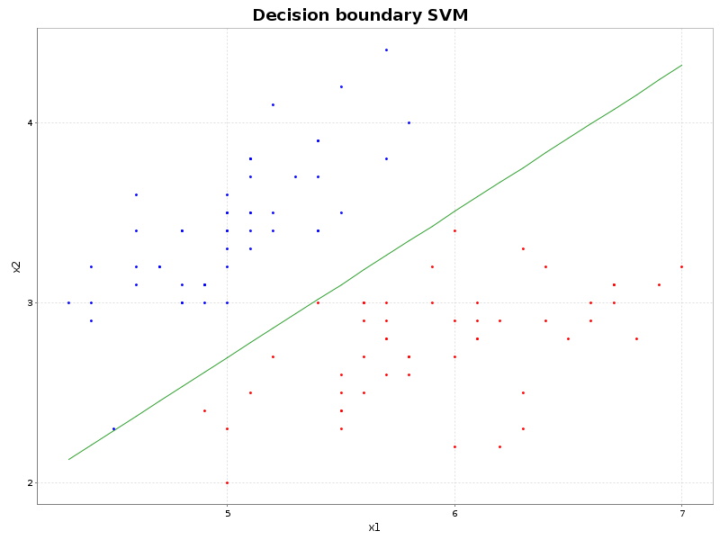
Decision boundary SVM object.
This post we discussed the definition of a linear support vector machine in a high level view. Next we defined the mathematical model of a SVM and finally we wrote a Scala class that is able to find an optimal hyperplane in linearly seperable data.
Further reads:
The model for the SVM discussed today is restricted to binary linearly seperable data only. If we want to classify non linearly seperable data, we need to attend to a technique called the kernel trick. If you want to classify more than two classes with a SVM, a commonly used method is one-vs-rest.
If you want to read a same kind of post about neural networks, read my earlier post.