Time series are a quite unique topic within machine learning. In a lot of problems the dependent variable $y$, i.e. the thing we want to predict is dependent on very clear inputs, such as pixels of an image, words in a sentence, the properties of a persons buying behavior, etc. In time series these indepent variables are often not known. For instance, in stock markets, we don’t have a clear independent set of variables where we can fit a model on. Are stock markets dependent on the properties of a company, or the properties of a country, or are they dependent on the sentiment in the news? Surely we can try to find a relation between those independent variables and stock market results, and maybe we are able to find some good models that map those relations. Point is that those relations are not very clear, nor is the independent data easily obtainable.
A common approach to model time series is to regard the label at current time step $X_{t}$ as a variable dependent on previous time steps $X_{t-k}$. We thus analyze the time series on nothing more than the time series.
One of the most used models when handling time series are ARIMA models. In this post, we’ll explore how these models are defined and we are going to develop such a model in Python with nothing else but the numpy package.
Stochastic series
ARIMA models are actually a combination of two, (or three if you count differencing as a model) processes that are able to generate series data. Those two models are based on an Auto Regressive (AR) process and a Moving Average process. Both AR and MA processes are stochastic processes. Stochastic means that the values come from a random probability distribution, which can be analyzed statistically but may not be predicted precisely. In other words, both processes have some uncertainty.
White noise
Let’s look at a very simple stochastic process called white noise. White noise can be drawn from many kinds of distributions. Here we draw from an univariate Gaussian.
$$ \epsilon \sim N(0, 1) $$
# fix some imports
import matplotlib.pyplot as plt
import seaborn as sns
import numpy as np
import scipy

n = 500
fig, ax = plt.subplots(1,2, figsize=(16, 6), gridspec_kw={'width_ratios':[3, 1]})
eps = np.random.normal(size=n)
ax[0].plot(eps)
sns.distplot(eps, ax=ax[1])
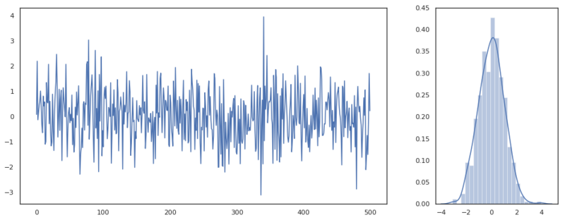
White noise signal.
This process is completely random, though we are able to infer some properties from this series. By making a plot of the distribution we can assume that these variables come from a single normal distribution with zero mean and unit variance. Our best guess for any new variables value would be the value 0. A better model for this process doesn’t exist as every new draw from the distribution is completely random and independent of the previous values. White noise is actually something we want to see on the residuals after we’ve defined a model. If the residuals follow a white noise pattern, we can be certain that we’ve declared all the possible variance.
MA process
A moving average process is actually based on this white noise. It is defined as a weighted average of the previous white noise values.
$$ X_t = \mu + \epsilon_t + \sum_{i=1}^{q}{\theta_i \epsilon_{t-i}} $$
Where $\theta$ are the parameters of the process and $q$ is the order of the process. With order we mean how many time steps $q$ we should include in the weighted average.
Let’s simulate an MA process. For every time step $t$ we take the $\epsilon$ values up to $q$ time steps back. First, we create a function that given an 1D array creates a 2D array with rows that look $q$ indices back.
def lag_view(x, order):
    """
    For every value X_i create a row that lags k values: [X_i-1, X_i-2, ... X_i-k]
    """
    y = x.copy()
    # Create features by shifting the window of `order` size by one step.
    # This results in a 2D array [[t1, t2, t3], [t2, t3, t4], ... [t_k-2, t_k-1, t_k]]
    x = np.array([y[-(i + order):][:order] for i in range(y.shape[0])])

    # Reverse the array as we started at the end and remove duplicates.
    # Note that we truncate the features [order -1:] and the labels [order]
    # This is the shifting of the features with one time step compared to the labels
    x = np.stack(x)[::-1][order - 1: -1]
    y = y[order:]

    return x, y
In the function above we create that 2D matrix. We also truncate the input and output array so that all rows have lagging values. If we call this function on an array ranging from 0 to 10, with order 3, we get the following output.
>>> lag_view(np.arange(10), 3)[0]

array([[0, 1, 2],
       [1, 2, 3],
       [2, 3, 4],
       [3, 4, 5],
       [4, 5, 6],
       [5, 6, 7],
       [6, 7, 8]])
Now we are able to easily take a look at different lags back in time. Let’s simulate three different MA processes with order $q=1$, $q=6$, and $q=11$.
def ma_process(eps, theta):
    """
    Creates an MA(q) process with a zero mean (mean not included in implementation).
    :param eps: (array) White noise signal.
    :param theta: (array/ list) Parameters of the process.
    """
    # reverse the order of theta as Xt, Xt-1, Xt-k in an array is Xt-k, Xt-1, Xt.
    theta = np.array([1] + list(theta))[::-1][:, None]
    eps_q, _ = lag_view(eps, len(theta))
    return eps_q @ theta

fig = plt.figure(figsize=(18, 4 * 3))
a = 310
for i in range(0, 11, 5):
    a += 1
    theta = np.random.uniform(0, 1, size=i + 1)
    plt.subplot(a)
    plt.title(f'$\\theta$ = {theta.round(2)}')
    plt.plot(ma_process(eps, theta))
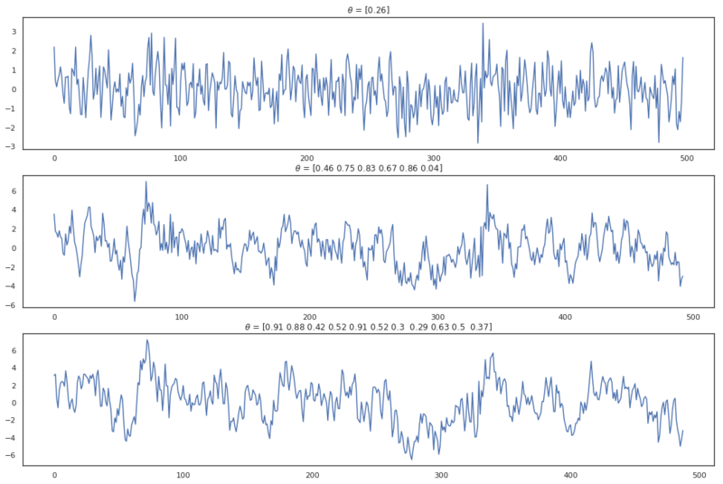
MA processes from different orders.
Note that I’ve chosen positive values for $\theta$ which isn’t required. An MA process can have both positive and negative values for $\theta$. In the plots above can be seen that when the order of MA(q) increases, the values are longer correlated with previous values. Actually, because the process is a weighted average of the $\epsilon$ values until lag $q$, the correlation drops after this lag. Based on this property we can make an educated guess on about order of an MA(q) process. This is great because it is very hard to infer the order by looking at the plots directly.
Autocorrelation
When a value $X_t$ is correlated with a previous value $X_{t-k}$, this is called autocorrelation. The autocorrelation function is defined as:
$$ACF(X_t, X_{t-k}) = \frac{E[(X_t - \mu_t)(X_{t-k} - \mu_{t-k})]}{\sigma_t \sigma_{t-k}}$$
Numerically we can approximate it by determining the correlation between different arrays, namely $X_t$ and array $X_{t-k}$. By doing so, we do need to truncate both arrays by $k$ elements in order to maintain an equal length.
def pearson_correlation(x, y):
    return np.mean((x - x.mean()) * (y - y.mean())) / (x.std() * y.std())

def acf(x, lag=40):
    """
    Determine autocorrelation factors.
    :param x: (array) Time series.
    :param lag: (int) Number of lags.
    """
    return np.array([1] + [pearson_correlation(x[:-i], x[i:]) for i in range(1, lag)])

lag = 40
# Create an ma(1) and an ma(2) process.
ma_1 = ma_process(eps, [1])
ma_2 = ma_process(eps, [0.2, -0.3, 0.8])
Above we have created an MA(1) and an MA(2) process with different weights $\theta$. The weights for the models are:
- MA(1): [1]
- MA(2): [0.2, -0.3, 0.8]
Below we apply the ACF on both series and we plot the result of both applied functions. We’ve also defined a helper function bartletts_formula which we use as a null hypothesis to determine if the correlation coefficients we’ve found are significant and not a statistical fluke. With this function, we determine a confidence interval $CI$.
$$CI = \pm z_{1-\alpha/2} \sqrt{\frac{1+2 \sum_{1 < i< h-1 }^{h-1}r^2_i}{N}} $$
where $ z_{1-\alpha/2} $ is the quantile function from the normal distribution. Quantile functions are the inverse of the cumulative distribution function and can be called with scipy.stats.norm.ppf. Any values outside of this confidence interval (below plotted in orange) are statistically significant.
def bartletts_formula(acf_array, n):
    """
    Computes the Standard Error of an acf with Bartlet's formula
    Read more at: https://en.wikipedia.org/wiki/Correlogram
    :param acf_array: (array) Containing autocorrelation factors
    :param n: (int) Length of original time series sequence.
    """
    # The first value has autocorrelation with it self. So that values is skipped
    se = np.zeros(len(acf_array) - 1)
    se[0] = 1 / np.sqrt(n)
    se[1:] = np.sqrt((1 + 2 * np.cumsum(acf_array[1:-1]**2)) / n )
    return se


def plot_acf(x, alpha=0.05, lag=40):
    """
    :param x: (array)
    :param alpha: (flt) Statistical significance for confidence interval.
    :parm lag: (int)
    """
    acf_val = acf(x, lag)
    plt.figure(figsize=(16, 4))
    plt.vlines(np.arange(lag), 0, acf_val)
    plt.scatter(np.arange(lag), acf_val, marker='o')
    plt.xlabel('lag')
    plt.ylabel('autocorrelation')

    # Determine confidence interval
    ci = stats.norm.ppf(1 - alpha / 2.) * bartletts_formula(acf_val, len(x))
    plt.fill_between(np.arange(1, ci.shape[0] + 1), -ci, ci, alpha=0.25)

for array in [ma_1, ma_2]:
    plot_acf(array)
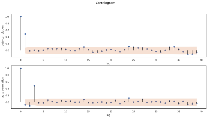
As we mentioned earlier, these plots help us infer the order of the MA(q) model. In both plots we can see a clear cut off in significant values. Both plots start with an autocorrelation of 1. This is the autocorrelation at lag 0. The second value is the autocorrelation at lag 1, the third at lag 2, etc. The first plot, the cut off is after 1 lag and in the second plot the cut off is at lag 3. So in our artificial data set we are able to determine the order of different MA(q) models by looking at the ACF plot!
AR process
In the section above we have seen and simulated an MA process and described the definition of autocorrelation to infer the order of a purely MA process. Now we are going to simulate another series called the Auto Regressive (RA) process. Again we’re going to infer the order of the process visually. This time we will be doing that with a Partial AutoCorrelation Function (PACF).
An AR(p) process is defined as:
$$X_t = c + \epsilon_t \sum_{i=1}^p{\phi_i X_{t-i}} $$
Now $\phi$ are the parameters of the process and $p$ is the order of the process. Where MA(q) is a weighted average over the error terms (white noise), AR(p) is a weighted average over the previous values of the series $X_{t-p}$. Note that this process also has a white noise variable, which makes this a stochastic series.
def ar_process(eps, phi):
    """
    Creates a AR process with a zero mean.
    """
    # Reverse the order of phi and add a 1 for current eps_t
    phi = np.r_[1, phi][::-1]
    ar = eps.copy()
    offset = len(phi)
    for i in range(offset, ar.shape[0]):
        ar[i - 1] = ar[i - offset: i] @ phi
    return ar

fig = plt.figure(figsize=(16, 4 * 3))
a = 310
for i in range(0, 11, 5):
    a += 1
    phi = np.random.normal(0, 0.1, size=i + 1)
    plt.subplot(a)
    plt.title(f'$\\phi$ = {phi.round(2)}')
    plt.plot(ar_process(eps, phi))
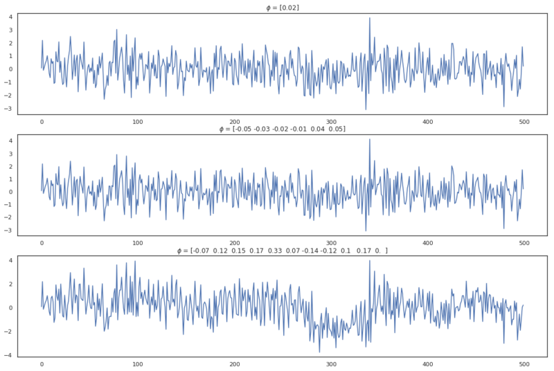
AR processes from different orders.
Below we create three new (AR(p) processes and plot the ACF of these series.
plot_acf(ar_process(eps, [0.3, -0.3, 0.5]))
plot_acf(ar_process(eps, [0.5, -0.1, 0.1]))
plot_acf(ar_process(eps, [0.2, 0.5, 0.1]))
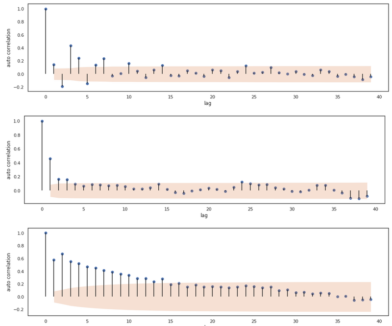
The ACF computed from 3 different AR series.
By analyzing these plots we can tell that the ACF plot of these AR processes don’t necessarily cut off after lag $p$. In the first plot, we see that the ACF values tail off to zero, the second plot does have significant cut off at lag $p$ and the third plot has a linearly decreasing autocorrelation until lag 14. For the AR(p) process, the ACF clearly isn’t decisive for determining the order of the process. Actually, for AR processes we can use another function for inferring the order of the process.
Partial autocorrelation
The partial autocorrelation function shows the autocorrelation of value $X_t$ and $X_{t-k}$ after the correlation between $X_t$ with the intermediate values $X_{t-1} … X_{t-k+1}$ explained. Below we’ll go through the steps required to determine partial autocorrelation.
The partial correlation between $X_t$ and $X_{t-k}$ can be determined by training two linear models.
Let $\hat{X_t}$ and $\hat{X_{t-k}}$ be determined by a Linear Model optimized on $X_{t-1} … X_{t-(k-1)} $ and parameterized by $\alpha$ and $\beta$.
$$\hat{X_t} = \alpha_1 X_{t-1} + \alpha_2 X_{t-2} … \alpha_{k-1} X_{t-(k-1)}$$
$$\hat{X_{t-k}} = \beta_1 X_{t-1} + \beta_2 X_{t-2} … \beta_{k-1} X_{t-(k-1)} $$
The partial correlation is then defined by the Pearson’s coefficient of the residuals of both predicted values $\hat{X_t}$ and $\hat{X_{t-k}}$.
$$ PCAF(X_t, X_{t-k}) = corr((X_t - \hat{X_t}), (X_{t-k} - \hat{X_{t-k}})) $$
Intermezzo: Linear model
Above we use a linear model to define the PACF. Later in this post, we are also going to train an ARIMA model, which is linear. So let’s quickly define a linear regression model.
Linear regression is defined by:
$$ y = \beta X + \epsilon $$
Where the parameters can be found by ordinary least squares:
$$ \beta = (X^TX)^{-1}X^Ty $$
def least_squares(x, y):
    return np.linalg.inv((x.T @ x)) @ (x.T @ y)

class LinearModel:
    def __init__(self, fit_intercept=True):
        self.fit_intercept = fit_intercept
        self.beta = None
        self.intercept_ = None
        self.coef_ = None

    def _prepare_features(self, x):
        if self.fit_intercept:
            x = np.hstack((np.ones((x.shape[0], 1)), x))
        return x

    def fit(self, x, y):
        x = self._prepare_features(x)
        self.beta = least_squares(x, y)
        if self.fit_intercept:
            self.intercept_ = self.beta[0]
            self.coef_ = self.beta[1:]
        else:
            self.coef_ = self.beta

    def predict(self, x):
        x = self._prepare_features(x)
        return x @ self.beta

    def fit_predict(self, x, y):
        self.fit(x, y)
        return self.predict(x)
Above we have defined a scikit-learn stylish class that can perform linear regression. We train by applying the fit method. If we also want to train the model with an intercept, we add ones to the feature matrix. This will result in a constant shift when applying $\beta X$.
With the short intermezzo in place, we can finally define the partial autocorrelation function and plot the results.
def pacf(x, lag=40):
    """
    Partial autocorrelation function.

    pacf results in:
        [1, acf_lag_1, pacf_lag_2, pacf_lag_3]
    :param x: (array)
    :param lag: (int)
    """
    y = []

    # Partial auto correlation needs intermediate terms.
    # Therefore we start at index 3
    for i in range(3, lag + 2):
        backshifted = lag_view(x, i)[0]

        xt = backshifted[:, 0]
        feat = backshifted[:, 1:-1]
        xt_hat = LinearModel(fit_intercept=False).fit_predict(feat, xt)

        xt_k = backshifted[:, -1]
        xt_k_hat = LinearModel(fit_intercept=False).fit_predict(feat, xt_k)

        y.append(pearson_correlation(xt - xt_hat, xt_k - xt_k_hat))
    return np.array([1, acf(x, 2)[1]] +  y)

def plot_pacf(x, alpha=0.05, lag=40, title=None):
    """
    :param x: (array)
    :param alpha: (flt) Statistical significance for confidence interval.
    :parm lag: (int)
    """
    pacf_val = pacf(x, lag)
    plt.figure(figsize=(16, 4))
    plt.vlines(np.arange(lag + 1), 0, pacf_val)
    plt.scatter(np.arange(lag + 1), pacf_val, marker='o')
    plt.xlabel('lag')
    plt.ylabel('autocorrelation')

    # Determine confidence interval
    ci = stats.norm.ppf(1 - alpha / 2.) * bartletts_formula(pacf_val, len(x))
    plt.fill_between(np.arange(1, ci.shape[0] + 1), -ci, ci, alpha=0.25)

plot_pacf(ar_process(eps, [0.3, -0.3, 0.5]))
plot_pacf(ar_process(eps, [0.5, -0.1, 0.1]))
plot_pacf(ar_process(eps, [0.2, 0.5, 0.1]))
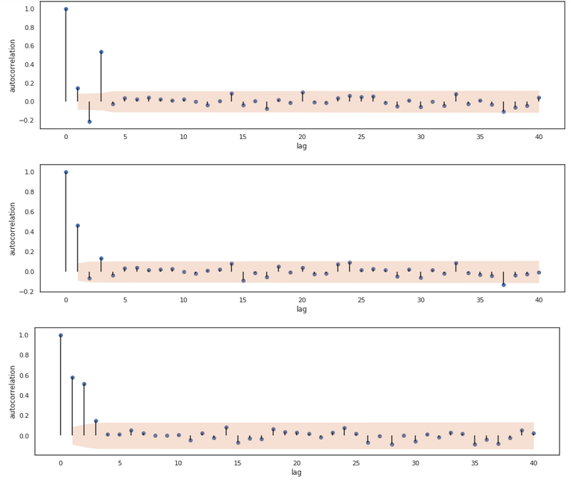
The PACF for 3 AR processes.
Now we see a significant cut off at lag 3 for all 3 processes! We thus are able to infer the order of the processes. The relationship between AR and MA processes and the ACF and PACF plots are one to keep in mind, as they help with inferring the order of a certain series.
| :) | AR(p) | MA(q) | ARMA(p, q) |
|---|---|---|---|
| ACF | Tails off | Cuts off after lag $q$ | Tails off |
| PACF | Cuts off after lag $p$ | Tails off | Tails off |
In the table above we show this relationship. The ARMA(p,q) process is also included in this table. We haven’t mentioned this process yet, but this is actutally just a combination of an AR(p) and an MA(q) series.
Before we go into this combination of AR and MA processes. We’ll go through one last definition, which is Integrated (the I in ARIMA). With that, we’ve touched all the parts of an ARIMA model.
Stationary
An ARMA model requires the data to be stationary, which an ARIMA model does not. A stationary series has a constant mean and a constant variance over time. For the white noise, AR and MA processes we’ve defined above, this requirement holds, but for a lot of real-world data this does not. ARIMA models can work with data that isn’t stationary, but instead has got a trend. For time series that also have recurring patterns (seasonality), ARIMA models don’t work.
When the data shows a trend, we can remove the trend by differencing time step $X_t$ with $X_{t-1}$. We can difference n times until the data is stationary. We can test stationarity with a Dicker Fuller test. How that is done is beyond the scope of this post.
We can difference a time series by
$$ \nabla X_t = X_t - X_{t-1} $$
and simply undo this by taking the sum
$$ X_t = \nabla X_t + \nabla X_{t-1} $$
We can easily implement this with two recurring functions.
def difference(x, d=1):
    if d == 0:
        return x
    else:
        x = np.r_[x[0], np.diff(x)]
        return difference(x, d - 1)

def undo_difference(x, d=1):
    if d == 1:
        return np.cumsum(x)
    else:
        x = np.cumsum(x)
        return undo_difference(x, d - 1)
ARIMA
Ok, finally we have discussed (and implemented) all topics we need for defining an ARIMA model. Such a model has hyperparameters p, q and, d.
- p is the order of the AR model
- q is the order of the MA model
- d is the differencing order (how often we difference the data)
The ARMA and ARIMA combination is defined as
$$ X_t = c + \epsilon_t + \sum_{i=1}^{p}{\phi_i X_{t - i}} + \sum_{i = 1}^q{\theta_i \epsilon_{t-i}} $$
We see that the model is based on white noise terms, which we don’t know as they come from a completely random process. Therefore we will use a trick for retrieving quasi-white noise terms. First, we will train the AR(p) model and then we will take the residuals as $\epsilon_t$ terms. Note that this will lead to an estimation of an ARIMA model. We could estimate the error terms $\epsilon$ more accurate by iteratively training the ARIMA model whilst updating the residuals every iteration. For now, we’ll accept the quasi-white noise method. With these white noise terms, we can start modelling the full ARIMA(q, d, p) model.
Below we’ve defined the ARIMA class which inherits from LinearModel. Because of this inheritage, we can call the fit and predict methods from the parent with the super function.
class ARIMA(LinearModel):
    def __init__(self, q, d, p):
        """
        An ARIMA model.
        :param q: (int) Order of the MA model.
        :param p: (int) Order of the AR model.
        :param d: (int) Number of times the data needs to be differenced.
        """
        super().__init__(True)
        self.p = p
        self.d = d
        self.q = q
        self.ar = None
        self.resid = None

    def prepare_features(self, x):
        if self.d > 0:
            x = difference(x, self.d)

        ar_features = None
        ma_features = None

        # Determine the features and the epsilon terms for the MA process
        if self.q > 0:
            if self.ar is None:
                self.ar = ARIMA(0, 0, self.p)
                self.ar.fit_predict(x)
            eps = self.ar.resid
            eps[0] = 0

            # prepend with zeros as there are no residuals_t-k in the first X_t
            ma_features, _ = lag_view(np.r_[np.zeros(self.q), eps], self.q)

        # Determine the features for the AR process
        if self.p > 0:
            # prepend with zeros as there are no X_t-k in the first X_t
            ar_features = lag_view(np.r_[np.zeros(self.p), x], self.p)[0]

        if ar_features is not None and ma_features is not None:
            n = min(len(ar_features), len(ma_features))
            ar_features = ar_features[:n]
            ma_features = ma_features[:n]
            features = np.hstack((ar_features, ma_features))
        elif ma_features is not None:
            n = len(ma_features)
            features = ma_features[:n]
        else:
            n = len(ar_features)
            features = ar_features[:n]

        return features, x[:n]

    def fit(self, x):
        features, x = self.prepare_features(x)
        super().fit(features, x)
        return features

    def fit_predict(self, x):
        """
        Fit and transform input
        :param x: (array) with time series.
        """
        features = self.fit(x)
        return self.predict(x, prepared=(features))

    def predict(self, x, **kwargs):
        """
        :param x: (array)
        :kwargs:
            prepared: (tpl) containing the features, eps and x
        """
        features = kwargs.get('prepared', None)
        if features is None:
            features, x = self.prepare_features(x)

        y = super().predict(features)
        self.resid = x - y

        return self.return_output(y)

    def return_output(self, x):
        if self.d > 0:
            x = undo_difference(x, self.d)
        return x

    def forecast(self, x, n):
        """
        Forecast the time series.

        :param x: (array) Current time steps.
        :param n: (int) Number of time steps in the future.
        """
        features, x = self.prepare_features(x)
        y = super().predict(features)

        # Append n time steps as zeros. Because the epsilon terms are unknown
        y = np.r_[y, np.zeros(n)]
        for i in range(n):
            feat = np.r_[y[-(self.p + n) + i: -n + i], np.zeros(self.q)]
            y[x.shape[0] + i] = super().predict(feat[None, :])
        return self.return_output(y)
Ok, let’s go through this one! As I’ve just mentioned, the ARIMA class inherits from LinearModel so first we initiate the parent and we pass the boolean True so that we also fit an intercept for the model. In the prepare_features method, (note that this one has no _ prefix and thus differs from the parent method) we create the features for the linear regression model. The features comprise of the lagging time steps $X_{t-k}$ with order q, which is
the AR part of the model, and of the lagging error terms $\epsilon_{t-k}$, which is the MA part of the model. In this method we also train an AR model first, so that we can use the residuals of that model as error terms.
Note that we prepend the $\epsilon$ and the $X$ with $n$ zeros, where $n$ is equal to order q and p respectively. This is done because there are no values $\epsilon_{t-q}$ and $X_{t-p}$ at time $X_0$. Furthermore, we just implement some methods inspired by scikit-learn naming conventions, e.g. the fit_predict, fit and predict methods.
We’ll discuss the forecast method later. Let’s first check how an object of the class is doing by comparing it with statsmodels implementation. We will also use test data coming from this library.
data = sm.datasets.sunspots.load_pandas().data
x = data['SUNACTIVITY'].values.squeeze()

plt.figure(figsize=(16,4))
plt.title('Sunspots')
plt.plot(x)
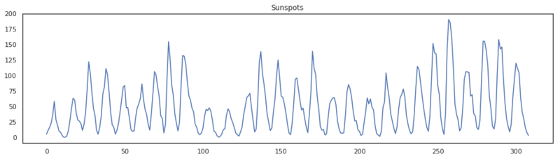
By the look of this data, it seems stationary. The mean and the variance don’t seem to be changing over time, so we can infer the first hyperparameter for this model. We don’t need to difference so d is set to 0. Let’s make an ACF and a PACF plot.
plot_acf(x)
plot_pacf(x)
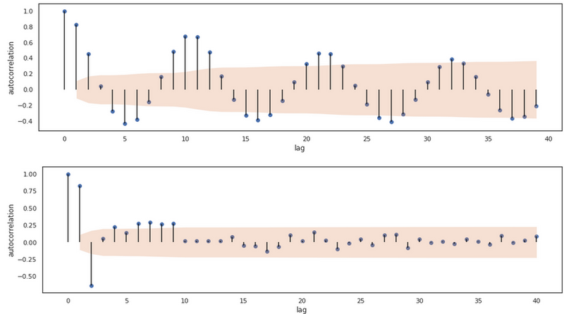
We see that the ACF clearly tails off and that the PACF tails a little bit, but seems to have a sort of cut off at lag 3. Based on this, let’s go for an ARIMA model with q=1, d=0, and p=3 and compare the model with the ARIMA implementation of statsmodels.
q = 1
d = 0
p = 3
m = ARIMA(q, d, p)
pred = m.fit_predict(x)
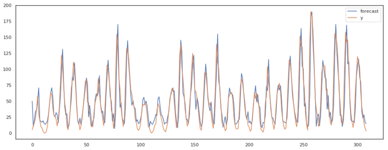
plt.figure(figsize=(16, 6))
ax = plt.subplot(111)
ax.plot(pred, label='forecast')
ax.plot(x, label='y')
plt.legend()
results = sm.tsa.ARIMA(x, (p, d, q)).fit()

plt.figure(figsize=(16, 6))
ax = plt.subplot(111)
pred_sm = results.plot_predict(ax=ax)
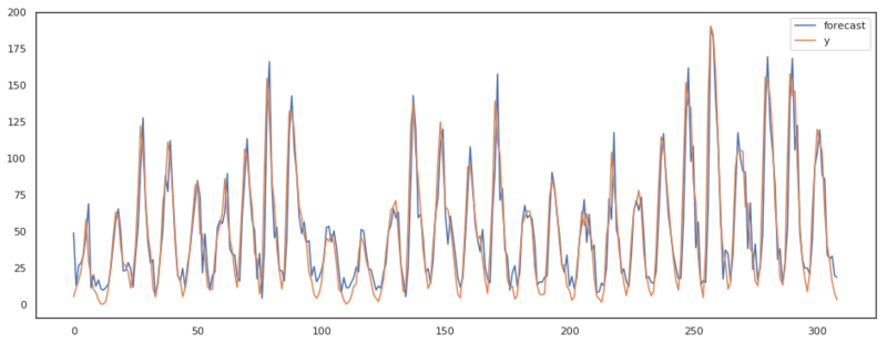
As we can see in the plots above, our ARIMA model has almost the same output as the implementation of statsmodels. There are some differences though. I assume these differences are present due to the fact that statsmodels keeps updating the residuals where we accepted the first residuals based on only the AR model.
Forecasting
There is one method we haven’t discussed, which is the forecast method. In this method we are trying to predict future values. By thinking about how we predict future values, we also see the weaknesses of this model. Because, as long as we have got labeled data points we can compute an error term $\epsilon_t$. However when we are making predictions, we don’t know the real data point $X_{t+k}$ and therefore we cannot compute the residuals. This means that after making
q (q being the order of the MA model) predictions, the ARMA model is only an AR model, as $E[\epsilon_{t+k}] = 0$ canceling out the weights of the MA model. The remaining AR model describes how the time series responds to a shock pushing $X_t$ from the mean value of the series.
Below we make a forecast of 40 time steps and we can clearly see the models response to the latest shock by tailing of to the mean of the series. This also shows the use case of this kind of model. It should be used for short term predictions. For long term predictions its output is just equal to the mean of the series.
pred = m.forecast(x, 40)
plt.figure(figsize=(12,4))
ax = plt.subplot(111)
ax.plot(x)
ax.plot(pred)
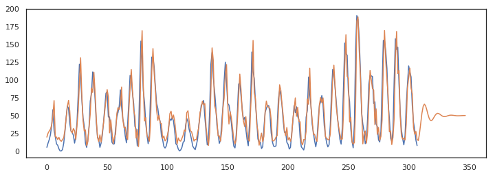
Forecasting with an ARMA model
Last words
We’ve discussed the definition of AR, MA, and ARIMA models in this post as well as the ACF and PACF. We’ve also come to the conclusion that these kind of models can only work with stationary data or data with a trend and that they are not suitable for long term forecasting. There is luckely an upgrade of the ARIMA model, called SARIMA. These models implement an ARIMA on p, d, and q and an addtional ARIMA on P, D, Q. The additional model works on the same time series, but then with a seasonal lag. For instance a seasonal lag of 4 would look like this
$$ X_{t}, X_{t-4}, X_{t-8} … X_{t-4k}$$
With this extension, the model is also more suitable for longer term predictions.
Do you wan’t to read more algorithm breakdowns? Take a look at: