Generative adversarial networks seem to be able to generate amazing stuff. I wanted to do a small project with GANs and in the process create something fancy for on the wall. Therefore I tried to train a GAN on a dataset of art paintings. This post I’ll explore if I’ll succeed in getting a full hd new Picasso on the wall. The pictures above give you a glimplse of some of the results from the model.
Generative Adversarial Networks
So what are those GANs actually? These networks are a different approach to monolithic neural networks. GANs are influenced by game theory. They consist of two networks, which compete with each other. One network, called the Discriminator, tries to identify the authenticity of an image. Another network, called the Generator, tries to fool the Discriminator by generating false images. The two networks are in an arms race and when this arms race is fruitful they will have learned to produce images that were not available to them in the dataset. The image below gives a visual explanation of what GANs are.
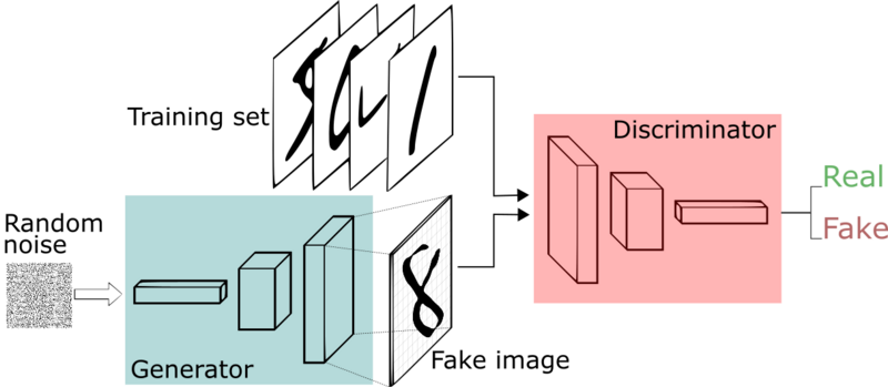
Generative Adversial networks
You see that we feed the Generator random noise. We sample this random noise from a normal distribution. We hope that through the magic of backpropagation the Generator will become a network that is able to transform this normal distribution to the actual distribution of the dataset.
That is right, the actual distribution of the dataset. Unlike models used for classification that model $P(class | data)$, GANs are able to learn and maximize $P(data)$ However GANs are notorious for being hard to train and instead of learning the latent distribution of a dataset they often learn just a small section of the hidden distribution or end up oscillating between only a few images during training.
Art data
Kaggle has a dataset containing the works of various painters. Shown below is an excerpt of the set. For the final dataset I’ve downloaded train_1.zip - train_6.zip.
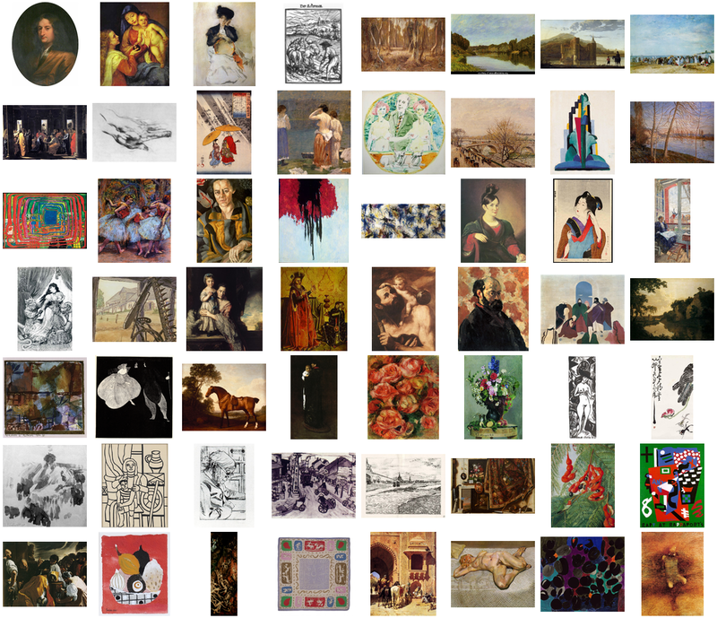
Some images from the dataset
Model
For this project I’ve used an architecture call Deep Convolutional Generative Adversarial Networks (DCGANs). The model is trained in Pytorch. The code is is included in this post. For the model to work, first import some dependencies.
import numpy as np
import torch
import torch.nn as nn
import torch.utils.data
import torch.nn.functional as F
import os
from torchvision import datasets, transforms
from PIL import Image
Discriminator
In this network the Discriminator is very much like any other deep convolutional network. It takes images as input and uses several feature extraction layers and finaly a fully connected layer to produce an output. The feature extraction layer is comprised of:
- Convolutional layer with 4x4 filters, a stride of 2 and a padding of 1 (downscaling an image by a factor 2).
- Batch normalization layer.
- Leaky relu activation.
The Discriminator outputs a Sigmoid activation where a threshold of 0.5 dictates the image being real or false.
class Discriminator(nn.Module):
    def __init__(self, alpha=0.2):
        super(Discriminator, self).__init__()

        kernel_size = 4
        padding = 1
        stride = 2

        self.net = nn.Sequential(
            nn.Conv2d(3, 128, kernel_size, stride, padding),
            nn.LeakyReLU(alpha),
            nn.Conv2d(128, 256, kernel_size, stride, padding),
            nn.BatchNorm2d(256),
            nn.LeakyReLU(alpha),
            nn.Conv2d(256, 512, kernel_size, stride, padding),
            nn.BatchNorm2d(512),
            nn.LeakyReLU(alpha),
            nn.Conv2d(512, 512, kernel_size, stride, padding),
            nn.BatchNorm2d(512),
            nn.LeakyReLU(alpha),
            nn.Conv2d(512, 512, kernel_size, stride, padding),
            nn.BatchNorm2d(512),
            nn.LeakyReLU(alpha),
            nn.Conv2d(512, 1024, kernel_size, stride, padding),
            nn.BatchNorm2d(1024),
            nn.LeakyReLU(alpha),
        )
        self.output = nn.Linear(4 * 4 * 1024, 1)

    def forward(self, x):
        x = self.net(x)
        x = torch.reshape(x, (-1, 4 * 4 * 1024))
        x = self.output(x)

        if self.training:
            return x

        return F.sigmoid(x)
Generator
The Generator is almost symmetrical to the Discriminator. But instead of convolutional layers that reduce the dimensionality of the image is upscaled using a transposed convolution. This convolution looks like this:
Transposed convolution. Input is blue, output is green.
The layers of the Generator are:
- Batch normalization layer
- Leaky relu activation
- Transposed convolutional layer with 4x4 filters, a stride of 2 and a padding of 1 (upscaling an image by a factor of 2)
class Generator(nn.Module):
    def __init__(self, input_size=200, alpha=0.2):
        super(Generator, self).__init__()
        kernel_size = 4
        padding = 1
        stride = 2

        self.input = nn.Linear(input_size, 4 * 4 * 1024)
        self.net = nn.Sequential(
            nn.BatchNorm2d(1024),
            nn.LeakyReLU(alpha),
            nn.ConvTranspose2d(1024, 512, kernel_size, stride, padding),
            nn.BatchNorm2d(512),
            nn.LeakyReLU(alpha),
            nn.ConvTranspose2d(512, 512, kernel_size, stride, padding),
            nn.BatchNorm2d(512),
            nn.LeakyReLU(alpha),
            nn.ConvTranspose2d(512, 512, kernel_size, stride, padding),
            nn.BatchNorm2d(512),
            nn.LeakyReLU(alpha),
            nn.ConvTranspose2d(512, 256, kernel_size, stride, padding),
            nn.BatchNorm2d(256),
            nn.LeakyReLU(alpha),
            nn.ConvTranspose2d(256, 128, kernel_size, stride, padding),
            nn.BatchNorm2d(128),
            nn.LeakyReLU(alpha),
            nn.ConvTranspose2d(128, 3, kernel_size, stride, padding),
            nn.Tanh()
        )

    def forward(self, z):
        x = self.input(z)
        return self.net(x.view(-1, 1024, 4, 4))
The output of the Generator is ran through a Tanh activation, squashing the output between -1 and 1. When we want to gaze at the creations in astonishment we rescale the output to integer values between 0 and 254 (RGB color values).
Preprocessing the data
The Discriminator is the only network that will perceive the real world art images. The images need to be rescaled to values between -1 and 1 to match the output of the Generator. For this we utilize some nice helper objects and functions from Pytorch.
class ImageFolderEX(datasets.ImageFolder):
    def __getitem__(self, index):
        def get_img(index):
            path, label = self.imgs[index]
            try:
                img = self.loader(os.path.join(self.root, path))
            except:
                img = get_img(index + 1)
            return img
        img = get_img(index)
        return self.transform(img) * 2 - 1  # rescale 0 - 1 to -1 - 1


trans = transforms.Compose([
    transforms.Resize((256, 256), interpolation=2),
    transforms.ToTensor(), # implicitly normalizes the input to values between 0 - 1.
])


# example showing how to use this helper object.
data = torch.utils.data.DataLoader(ImageFolderEX('.', trans),
	batch_size=64, shuffle=True, drop_last=True, num_workers=0)
x = next(iter(data))
Training
There are various tactics for stabilizing GAN training. The tricks I used to stabilize the learning of the networks are:
- Sampling the random input vector $z$ from a Gaussian instead of a Uniform distribution.
- Construct different mini-batches for real and fake data (i.e. not shuffling the real and fake in one mini-batch).
- Soft labels for the Discriminator (preventing the discriminator to get too strong) Salimans et. al. 2016.
- Occasionally swap the labels for the Discriminator (preventing the discriminator to get too strong).
- Use Adam hyperparameters as described by See Radford et. al. 2015.
Those stabilizing tricks are implemented in the different training functions for the Generator and the Discriminator.
def train_dis(dis, gen, x):
    z = torch.tensor(np.random.normal(0, 1, (batch_size, 200)), dtype=torch.float32)

    if next(gen.parameters()).is_cuda:
        x = x.cuda()
        z = z.cuda()

    dis.zero_grad()
    y_real_pred = dis(x)

    idx = np.random.uniform(0, 1, y_real_pred.shape)
    idx = np.argwhere(idx < 0.03)

    # swap some labels and smooth the labels
    ones = np.ones(y_real_pred.shape) + np.random.uniform(-0.1, 0.1)
    ones[idx] = 0

    zeros = np.zeros(y_real_pred.shape) + np.random.uniform(0, 0.2)
    zeros[idx] = 1
    ones = torch.from_numpy(ones).float()
    zeros = torch.from_numpy(zeros).float()

    if next(gen.parameters()).is_cuda:
        ones = ones.cuda()
        zeros = zeros.cuda()

    loss_real = F.binary_cross_entropy_with_logits(y_real_pred, ones)

    generated = gen(z)
    y_fake_pred = dis(generated)

    loss_fake = F.binary_cross_entropy_with_logits(y_fake_pred, zeros)
    loss = loss_fake + loss_real
    loss.backward()
    optimizer_dis.step()
    return loss


def train_gen(gen, batch_size):
    z = torch.tensor(np.random.normal(0, 1, (batch_size, 200)), dtype=torch.float32)

    if next(gen.parameters()).is_cuda:
        z = z.cuda()

    gen.zero_grad()
    generated = gen(z)
    y_fake = dis(generated)

    ones = torch.ones_like(y_fake)
    if next(gen.parameters()).is_cuda:
        ones = ones.cuda()

    loss = F.binary_cross_entropy_with_logits(y_fake, ones)
    loss.backward()
    optimizer_gen.step()
    return loss, generated
Now with all the models, preprocessing and training functions defined we can start the training loop.
dis = Discriminator().cuda()
gen = Generator().cuda()

lr = 0.0002
beta_1 = 0.5
beta_2 = 0.999
optimizer_gen = torch.optim.Adam(gen.parameters(), lr, betas=(beta_1, beta_2))
optimizer_dis = torch.optim.Adam(dis.parameters(), lr, betas=(beta_1, beta_2))

epochs = 20
batch_size = 64
data = torch.utils.data.DataLoader(ImageFolderEX('.', trans),
				   batch_size=batch_size, shuffle=True,
				   drop_last=True, num_workers=2)

n = len(data)
for epoch in range(0, epochs):
    c = 0
    n = len(data)

    for x in iter(data):
        c += 1

        loss_dis = train_dis(dis, gen, x)
        loss_gen, generated = train_gen(gen, batch_size)

        global_step = epoch * n + c

        if c % 4 == 0:
            print(f'loss: {loss_dis.item()}, \t {loss_gen.item()} \t epoch: {epoch}, \t {c}/{n}')
Results
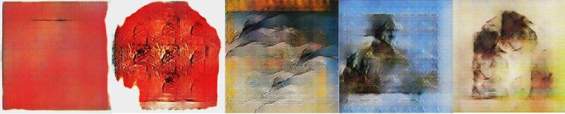
I’ve run two different variations of the GAN architecture described above. One that produces images with a resolution of 256x256 pixels and one that produces 64x64 images. The 256 pixel architecture produced the images shown below.
256x256 GAN
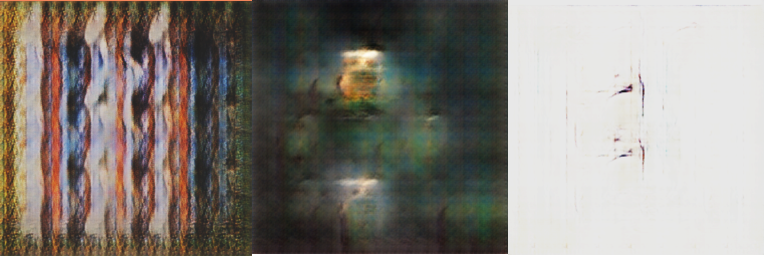
Images produced by the 256x256 GAN.
This variant was less stable in learning than the 64 pixel variant. The distribution of the images produced by this variant has got a lot less variance than the smaller network. Because of this smaller variance, I had to cherry pick the images at different weight configurations of the network.
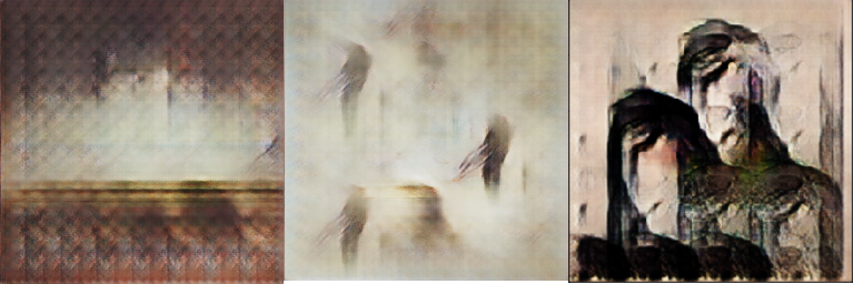
64x64 GAN
With the 64x64 architecture this isn’t the case. The network has captured a distribution with a lot more variation in both the images and the pixels.
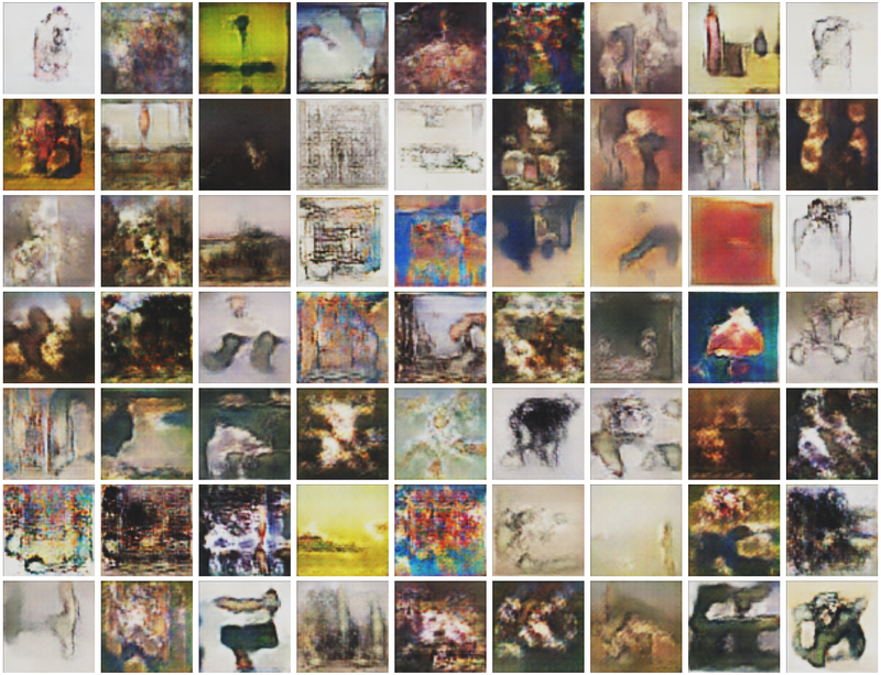
Images produced by the 64x64 GAN.
T. White et. al. described a way of interpolating the manifold of the Gaussian input we sample. By interpolating the input vectors and thereby following the curve of the manifold we can see how one image morphs in another. This is really cool! The method called slerp (spherical linear interpolation) is defined by:
where
- $\theta$ = angle between the two vectors.
- $\mu$ = interpolation factor between 0 and 1.
In the visual below we’re taking a small trip through the latent space of the 64x64 architecture.
Small trip around the distribution.
Final words
The generated images produced some really nice colors and shapes and in my opinion both network architectures learned the conditional probability of colors in art painings. Both networks didn’t produce any sharp figurative image. I believe that this is harder and needs a more consistent dataset, for instance images containing only painting of flowers.
My budget for the cloud gpu’s has run out, thus sadly my final conclusion is that the generated art on my wall at home won’t be in full-hd just yet.