Introduction
As a nerd I am fascinated by the deep learning hype. Out of interest I have been following some courses, reading blogs and watched youtube video’s about the topic. Before diving into the content, I really thought this was something solely for the great internet companies and that it was not a subject us mortals could understand.
While reading and learning more about it I’ve come to the insight that making use of deep learning techniques is not only something the internet giants and scientists can do. Thanks to the open source development of the machine learning community and technological advancement, open source deep learning libraries are now available for everybody with a reasonable computer to play and tinker with.
Just for fun and learning purposes, I am trying to make a music classifier with different deep learning algorithms. In multiple posts I will share my insights, choices, failures, results, and if I am really hyped maybe even my emotions. But the latter I won’t promise.
This first post focusses on the data retrieval and feature extraction. Before training any neural net on the data I will examine the data distribution.
## Data
As learning is all about experience, we need to let a machine experience. This is done in the form of data. I want to make use of supervised learning techniques. That means the data also needs to be labeled. Labeled means that a jazz song is labeled as, well, a jazz song. I don’t feel like hitting the record button on my soundblaster stereo every time a jazz song may be played. Therefore I have used the Spotify web api. I found they have got playlistst that are (somewhat) ordered by genre.
Before you can use the Spotify web api, you need to create a developers account. After doing so they will provide you with a client id and a secret token. You can create an account here.
I’ve made a notebook that will download the music for you. Of course there are some legal limitations to downloading music, thereore you only get a preview of the song from Spotify. The preview songs have a duration of 30 seconds. Most of the time we can classify a song by genre in less than 5 seconds so the 30 seconds duration is probably long enough for a neural net to classify our songs.
Run this notebook to start your 30 seconds disco!
Images
After some research I learned that most people who also played with music and neural nets did not feed raw audio into the networks. Most of the neural nets excel in recognizing images. To utilize this property I’ve used techniques in speech recognition and sound processing to downgrade the dimensionality and extract important features from the raw music data. The results are saved as images. In the text below I describe which features were extracted from the raw audio.
Mel spectogram
We can get frequency information of a song by taking the Fourier transform (FFT) of the signal. Read more about Fourier in my earlier post. However by doing so we trade all time information into frequency information, which is a huge loss of information.
The solution to this problem is quite simple however. Instead of doing a FFT over the whole time signal, it is done in discrete time steps. At every time step dt you will get frequency information.
Normally when doing an FFT, the frequency is plotted on the x-axis. Now the frequencies will be plotted on the y-axis. The result is called a spectogram, which is time and frequency information of an audio signal. The y-axis isn’t plotted in linear scale, but in Mel scale. A Mel scale is defined by the way we humans hear. Every increment on the Mel scale sounds equally apart to us humans. What we are actually doing is extracting features that are important to us humans. As we are also the species that define which music belongs to which genre. So I don’t know yet if this works, but this seems like a rational thing to do.
Below are some of the spectograms shown. The x-axis shows the duration of the song in seconds. The y-scale is the Mel scale and shows the frequencies as we hear them as humans. The color intensity shows the magnitude of the frequency. Where yellow/orange is intense and black is the absence of te frequency. I like these images as we could really tell something about the songs tunes. Furthermore you can notice that even in an image form EDM is way too intense.
The notebook used to convert the mp3 files to images can be found here
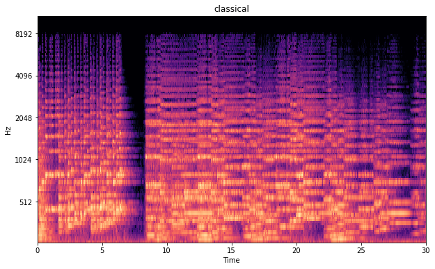
Mel spectogram classical music
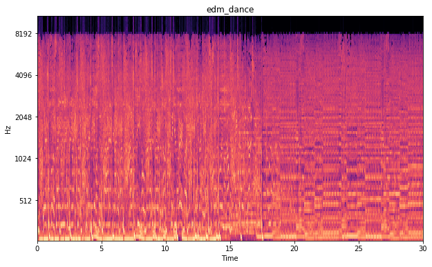
Mel spectogram electronic dance
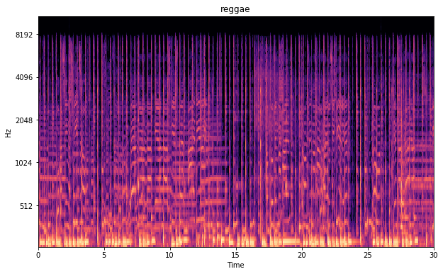
Mel spectogram reggae
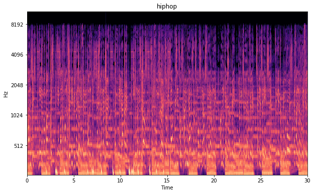
Mel spectogram hiphop
MFCC
To further reduce dimensionality of the music, I have also made Mel frequency cepstral coefficients(MFCC) images from the data. It is a processing technique commonly used for algorithms used for speech recognition. Just like the Mel spectograms this is feature extraction. Oversimplifying an MFCC could be seen as a spectrum of volume coefficients inspired by the way we humans hear, such as in the case with the Mel spectogram. This stackexchange answer gives a clear description of what MFCC’s are.
The image below shows an MFCC of a jazz song. It seems to me that this isn’t something that is meant to be readible by humans. To be sure that a machine is able to recognize something in this data I’ve done a principal component analysis on the MFCC images. This is described in the text below.
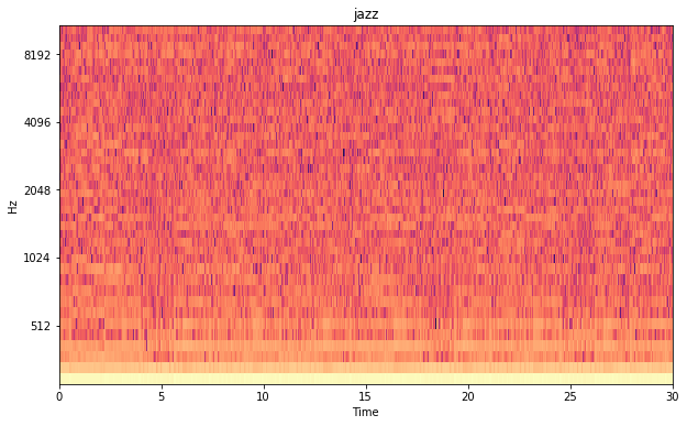
MFCC jazz
Principal components
Before doing any machine learning with the data I want to know how these images would be clustered if we reduce the dimensions. For this purpose I utilize the Principal Component Analysis. PCA is a statiscal procedure that returns principal components of parameters with the highest variance. Think of a principal component as an axis vector on which you can project the data. The first principal component will follow the axis on which the data shows the highest variance. The second principal component is perpendical on that axis and shows the second highest variance.
If there are N dimensions in your data there are also N principal components. The last principal components show the least variance and are least significant. In other words they give you little information about how to classify the data.
The figure below shows the two pincipal components of a distribution.
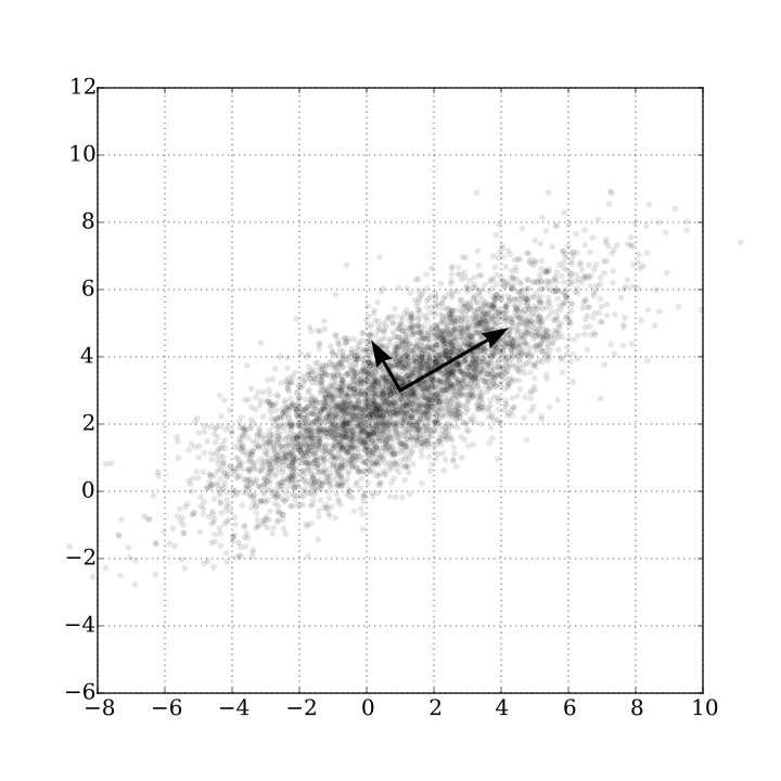
Two principal components of a distribution
Clustering
Note that I dropped some genres. After downloading I concluded that most of the genres data was really ambiguous. The rock dataset had a lot of numbers that could be regarded hiphop or soul and vice versa. Therefore I’ve chosen to continue with the genres that in my opinion were most distinctive or had the most data. The winning genres are:
- hiphop
- EDM
- classical
- metal
- jazz
The winning genres were rewarded with a principal component analyis. Below is the result plot shown of the principal component analysis. The analysis is done on the MFCC images. The different genres are already somewhat clustered, even before applying any machine learning algorithm on the data. Metal and classical music seem to be pretty distinctive music. EDM seems to have some overlap with jazz and hiphop. Based on this plot I would say it would be hardest for the learning algorithm to distinguish between jazz, hiphop and EDM.
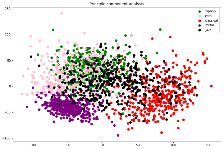
Principal component plot Mel spectogram images
I really think the image above is amazing. I could not believe that we get such a nice clustering in two dimensions from something so complicated and high dimensional as music. It is really interesting that it pretty much seems to coincide with my definition of the music genres.
This post described how I got the music data and how extracted important features (for us humans) from it. Next post I am going to feed this data to some different neural nets. Stay tuned.
TL;DR
I am trying to build a music classifier with deep learning models. I’ve downloaded some labeled music from spotify and converted it into images. I was really surprised by the way the data clustered afer doing a principal component analysis.
Next post I am going to try to predict some genres with different multi layer perceptron models.