For a project at Xomnia, I had the oppertunity to do a cool computer vision assignment. We tried to predict the input of a road safety model. Eurorap is such a model. In short, it works something like this. You take some cars, mount them with cameras and drive around the road you’re interested in. The ‘Google Streetview’ like material you’ve collected is sent to a crowdsourced workforce (at Amazon they are called Mechanical Turks) to manually label the footage.

Workforce labeling images of Dutch Roads.
This manually labeling of pictures is of course very time consuming, costly, not scalable and last but not least boooring!
Just imagine yourself clicking through thousands of images like the one shown below.
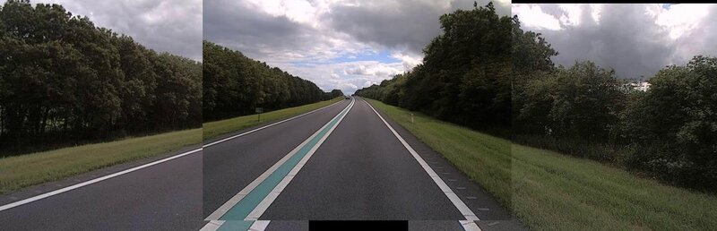
The thrilling working life of a mechanical Turk.
This post describes the proof of concept we’ve done, and how we’ve implemented it in Pytorch.
Dataset
The video material is divided in images shot every 10 meters. Even a Mechanical Turk has trouble not shooting itself of boredom when he has to fill in 300 labels of what he sees every 10 meters. To make his work a little bit more pleasant he only had to fill in the labels every 100 meter for what they had seen in the 10 pictures.
This working method has led to terrible labeling of the footage however. Every object that you drive by within these 100 meters is labeled to all 10 images, whilst it most of the time only is visible in 2~4 images!
We did a proof of concept and we’ve only regarded a small subset of all labels. In total there are approximately 300. We have done our analysis on 28 labels. And because of the problem of the mislabeled objects, we’ve chosen mostly labels that are visible parallel to the road. As it seems likely that those labels hold true for all 10 images. For instance, a road that has emergency lane in one image, is likely to have an emergency lane in the subsequent images.
Below you’ll see a plot with the labels we have trained our model on, and the amount of occurrences of that specific label. In total there were approximately 100,000 images in our dataset.
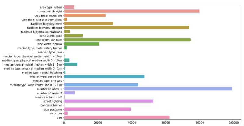
Counts of the labels we've used.
Transfer learning
There is a reasonable amount of images to work with, however the large inbalance in the labels, the errors in the labeling, and the amount of data required for the data hungry models called neural networks make it unlikely that we have enough data to properly train a robust computer vision model.
To give you an idea of the scale here. The record breaking convolutional neural networks, you read about in the news, are often trained on the imageNet dataset, which contains 1.2 million images. These modern ConvNets (convolutional neural networks) are trained for ~2 weeks on heavy duty GPU’s to go from their random initialization of weights, to a configuration that is able to win prices.
It would be nice if we don’t have to waste all this computational effort and somehow could transfer what we have learned in one problem (imageNet) to another (roadImages). Luckely, with ConvNets this isn’t a bad idea and there is quite some logical intuition in doing so. Neural networks are often regarded as black box classifiers. And for the classification part, this is currently somewhat true. But for traditional ConvNet architectures there is a clear distinction between the classification and the feature extraction.
And this feature extraction part is:
- Not so black box at all.
- Very transferable.
Not so black box at all
When taking a look at which pixels of an image result in activations (i.e. neurons having a large output) in convolutional layers, we can get some intuition on what is happening and meant with feature extraction.
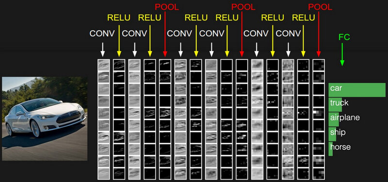
Feature extraction.
When we look at the activated neurons in the first layers, we can clearly identify the car. This means that there are a lot of low level features activated. Even so much that we can still identify the car in the activated neurons. The lower level features are for instance, edges, shadows, textures, lines, colors, etc.
Feature extractions in the first layer.
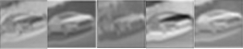
Based on these activations of lower features, new neurons will activate, growing in hierarchy and complexity. Activated edges combine in activations of curves, which can on itself in combination with other features lead to activations of objects, like a tyre or a grill. Lets say that in the image above a neuron is highly activated because a complex feature like a car grill. We wouldn’t be able to see this in an image of the activations. As there is only one grill in car (and one grill detector in our network), we would only see one activated neuron, i.e. one white pixel!
Feature extractions in the last layer.
Very transferable
Continuing in this line of thought, it seems pretty reasonable to assume that these lower level features extend to more objects than cars. Almost every picture has got edges, shadows, colors and so forth. This means that a lot of the weigths in the feature extraction neurons in a price winning ConvNet are set just right, or at least close by, to our wanted configuration of the weights.
This works so well, that we can pretrain a ConvNet on a large dataset like ImageNet and transfer the ConvNet to a problem with a relatively small dataset (that normally would be insufficient for this ConvNet architecture). The pretrained model still needs to be finetuned. There are a few options like freezing the lower layers and retraining the upper layers with a lower learning rate, finetuning the whole net, or retraining the classifier.
In our case we finetuned the feature extraction layers with low learning rates, and changed the classifier of the model.
Implementation
For this project we’ve tried various pretrained ConvNet architectures like GoogleNet, ResNet and VGG and found VGG to produce the best result, closely followed by ResNet. In this section we’ll go through the VGG implementation in Pytorch.
import torch
import torch.nn as nn


class VGG(nn.Module):
    def __init__(self):
        num_classes = 1000
        super(VGG, self).__init__()
        self.features = self.make_layers([64, 'M', 128, 'M', 256, 256, 'M', 512, 512, 'M', 512, 512, 'M'])
        self.classifier = nn.Sequential(
            nn.Linear(512 * 7 * 7, 4096),
            nn.ReLU(True),
            nn.Dropout(),
            nn.Linear(4096, 4096),
            nn.ReLU(True),
            nn.Dropout(),
            nn.Linear(4096, num_classes),
        )

    def make_layers(self, cfg):
        layers = []
        in_channels = 3
        for v in cfg:
            if v == 'M':
                layers += [nn.MaxPool2d(kernel_size=2, stride=2)]
            else:
                conv2d = nn.Conv2d(in_channels, v, kernel_size=3, padding=1)
                layers += [conv2d, nn.BatchNorm2d(v), nn.ReLU(inplace=True)]
                in_channels = v
        return nn.Sequential(*layers)
Shown above is the a base implementation of a pretrained VGG net with 11 layers and batch normalization. The feature extraction part of VGG is cfg variable we pass to the make_layers method. The list [64, 'M', 128, 'M', 256, 256, 'M', 512, 512, 'M', 512, 512, 'M'] describes the architecture, with the integers being the depth of the convolution channels, and M being a maxpooling layer to reduce dimensionality.
As you can see we’ve still defined a classifier with 1000 classes (# of classes in ImageNet) in the model, even though I’ve just mentioned that we would change that. We need the original model to be able to load the state_dict (dictionary containing al the weights and biases of the pretrained model) and load the weights and biases.
This pretrained model is of course not suitable for our problem, therefore we will define another class which will enbody the model we need for our problem.
class VGGmod(nn.Module):
    def __init__(self, h, dropout):
        super(VGGmod, self).__init__()
        model = VGG()
        model_pretrained.load_state_dict(
            model_zoo.load_url(model_urls['https://download.pytorch.org/models/vgg11_bn-6002323d.pth']))
        self.features = model.features
        self.classifier = nn.Sequential(
            nn.Linear(25088, h),
            nn.ReLU(inplace=True),
            nn.Dropout(dropout),
            nn.Linear(h, h),
            nn.ReLU(inplace=True),
            nn.Dropout(dropout),
            nn.Linear(h, 28)
        )

    def forward(self, x):
        x = self.features(x)

        # view is a resizing method
        x = x.view(x.size(0), -1)  # -1 means infer the shape based on the other dimension
        x = self.classifier(x)

        # area type
        a = F.sigmoid(x[:, 0])
        # curvature
        b = F.softmax(x[:, 1: 4], dim=1)
        # facilities for bicycles
        c = F.softmax(x[:, 4: 7], dim=1)
        # lane width
        d = F.softmax(x[:, 7: 10], dim=1)
        # median type
        e = F.softmax(x[:, 10: 20], dim=1)
        # number of lanes
        f = F.softmax(x[:, 20: 23], dim=1)
        # rest
        g = F.sigmoid(x[:, 23:])

        return torch.cat([a.unsqueeze(-1), b, c, d, e, f, g], dim=1)


model = VGGmod(300, 0.5)
Above we’ve defined the final model. At initialization we assign the pretrained VGG-net to model and we copy its feature extraction layers at self.features = model.features.
Combined output layer
The model has to classify various objects in a picture. Some objects can always be in the picture, whilst others are mutually exclusive. The presence of one object means that another cannot be present. There can for instance be only one type of median type in the picture. To implement this constraint there are different activations functions applied to different parts of the output vector. The objects that are not restricted by the presence of other objects (tree, street light, etc.) are activated by a sigmoid function. The mutually exclusive objects (types of curvature, types of bicycle facilities, etc.) are activated by a softmax function. This way the dependence is learned through backpropagation.
In the last part of the model this special output vector is implemented in the classifier consisting of two fully connected layers with Relu activation, dropout, and finally the output vector.
The output vector and the different activations are shown below.

The different activations on the final output vector.
Loss function
This mutually exclusive constraint could also be implemented in the loss function by using a Binary Crossentropy loss on the sigmoids and a normal Crossentropy loss on the softmax and summarizing the outputs. However we’ve learned that the lazy implementation worked quite well. We’ve used a Binary Crossentropy loss on the whole output vector.
Results
Shown below are the results of the training effort. The horizontal axis shows the recall score of the labels, and the vertical axis the precision. It is often an exchange of those metrics, where scoring better on one, reduces the score of the other. The optimal spot is in the upper right corner.
The size of the scatter dots are proportional to the amount of labels in the dataset. Unsurprisingly we can see a correlation with the number of labels and the final score.
I am quite pleased with the results however. Especcially knowing that a lot of the data is mislabeled. The model gained high scores on number of lanes: 2, facilities bicycles: on-road lane, median type: metal safety barrier. All labels that weren’t abundantly available in the dataset.
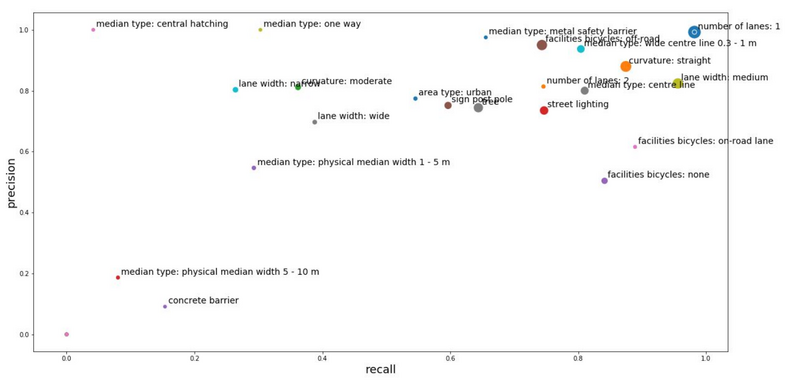
Results of the different labels
Some inference of the model. Below are some random classification results shown. Note: the absence of a median type is labeled as median type: centre line in the dataset.
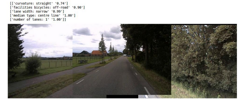
Random inference sample.
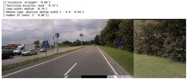
Random inference sample.
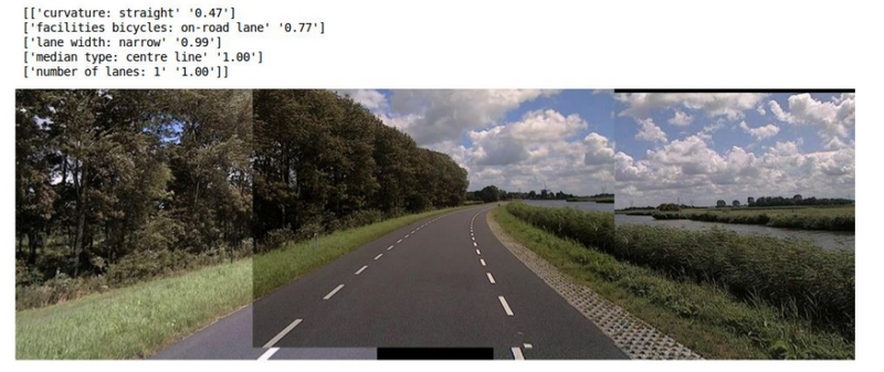
Random inference sample.
Conclusion
This project we’ve seen the effectiveness of transfer learning. Though the dataset was quite dirty and had a lot of flawed labels, the proof of concept was successfull.
By using a model pretrained on imageNet, the final model seemed robust and was able to successfully learn the features that were sufficiently available in the dataset. The other features are certainly learnable, but would require some hand labeling the future. The feasibility of this hand labeling is something that is being researched at the moment. So, who knows. Maybe there will be a follow up on this post in the future!