
This is post was a real eye-opener for me with regard to the methods we can use to train neural networks. A colleague pointed me to the SLIDE[1] paper. Chen & et al. discussed outperforming a Tesla V100 GPU with a 44 core CPU, by a factor of 3.5, when training large neural networks with millions of parameters. Training any neural network requires many, many, many tensor operations, mostly in the form of matrix multiplications. These tensor operations are often offloaded to GPU’s or TPU’s. This kind of hardware is specifically designed to do matrix multiplications in parallel. Originally just to render games/ videos. But in the latest years they have also found their use in neural network training and crypto mining. GPU’s are very fast and I believe the current AI hype wouldn’t be here if we had to run all algorithms on the CPU.
However, a neural network does a lot of wasted computation. Imagine a simple layer with a ReLU activation. $\text{ReLU}(w^Tx + b) = \max(0, w^Tx + b)$. Any negative output of a neuron was a wasted computation as the result is nullified. The SLIDE paper discusses methods to reduce the wasted computation by only computing the activated neurons (with a high probability). This post we’ll take a look at those methods. If you need a refreshment on the inner workings of neural networks, I’d recommend an earlier post on this subject.
1 NN ♥ hash tables
Instead of computing all neurons in all layers. We could throw layer inputs in hash function and lookup wich neurons probably will be activated. At first, this may sound a bit like magic. How can there exist a hash function that points us to the activated neurons? Let’s first have some introduction on hash functions.
1.1 Hash functions
A hash function is often used in computer science to achieve $\mathcal{O}(1)$ lookup complexity. Formaly a hash function takes an input of variable length and maps to an output of constant length. This output is then often used as a pointer that refers to some data storage location. The location the hash value points towards is called a bucket. The bucket can contain one single value, or when some hashes collide (point to the same bucket) it has multiple unique values. The figure below shows an example of a hash function that maps to different buckets.
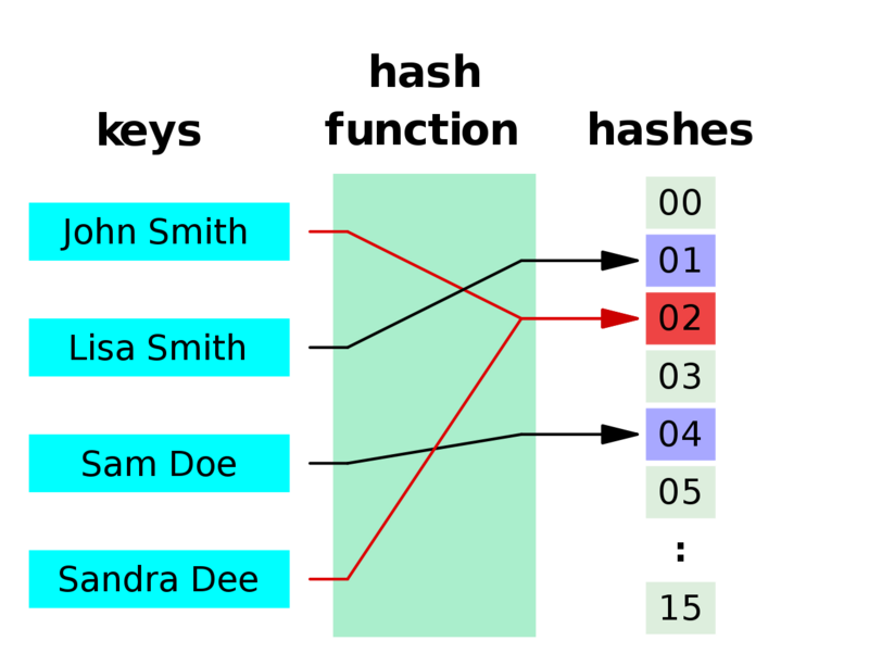
A visual example of a hash function.
Hashes are also common in cryptography. These hash functions have the property that a subtle change in the input leads to an entirely different hash value. An example of this is the md5 checksum often done on file contents. The code snippet below shows an example in Python.
First, we hash the string value; "somestring", and next we hash a very similar string; "somestrinG". Although the input strings are very similar, the hashed outputs are very different.
import hashlib
hashlib.md5(b"somestring").hexdigest()
>>> '1f129c42de5e4f043cbd88ff6360486f'
hashlib.md5(b"somestrinG").hexdigest()
>>> '941845035b4bfa672cc6803598b1fe87'
1.2 Collisions
Most hash functions we encounter are designed with a low collision probability. However, in our case we would like to find a hash function that maximizes the collision probability for certain cases. Below we’ll discuss why.
The figure below shows an artifical neuron. One of many in a neural network.
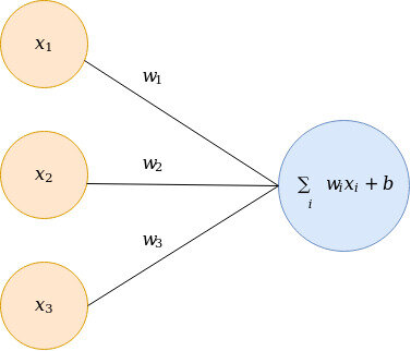
Neuron in a neural network.
The most expensive, and important, operation in a single neuron is the inner product: $w^T x$. So let’s reiterate the goal here. Many of those neurons is a network don’t activate (here I regard a low activation as a non-activation), and thus the computation was a waste of effort. Ideally, we only want to compute the neurons that activate and ignore the remaining neurons. Neurons activate when the inner product $w^Tx » 0$. We would like to obtain a hash function that collides with high probability if two vectors have a large inner product, i.e. the neuron activates. So more formally; $P(h(x) = h(w))$ is maximized when $w^Tx$ is large, where $h(\cdot)$ is a hash function $h: \mathbb{R}^m \mapsto \mathbb{R}^n$.
One of the many ways we can measure the similarity between two vectors of equal dimension size is cosine similarity. Let $A \in \mathbb{R}^D$ and $B \in \mathbb{R}^D$, cosine similarity is defined as:
$$ \cos(\theta) = \frac{A \cdot B}{ \left| \left| A \right| \right| \left| \left| B \right| \right| } $$
The dot product, $\sum_{i=1}^n A_i B_i$, in the numerator has the property that similar signed indexes in the vector lead to positive signed output values. That means that vectors with many similar signed indexes will likely have a positive dot product, $A \cdot B > 0$, and vectors where the signs differ much will likely have a negative dot product, $A \cdot B < 0$. The denominator is a normalizing factor and scales the dot product to $-1 \leq \cos(\theta) \leq 1$. Where values close to 1 are thus very similar, and values close to -1 are very opposite vectors.
As mentioned above, the main operation in a single neuron is a dot product $w \cdot x$, there is no normalizing factor $ \left| \left| w \right| \right| \left| \left| x \right| \right| $. So from a purely mathematical point of view, the cosine similarity doesn’t fit as similarity function to find the activating neurons. However, from a pragmatic point of view, it does. The weights and inputs of a neural network are often normalized such that $E[w] = 0$, and $\text{Var}(w) = 1$. This will make most normalizing factors approximately similar, and therefore less important.
Another pragmatic reason we choose cosine similarity is that it easier to find a hashing function that will maximize $P(h(x) = h(w))$ for similar vectors.
2 Locality Sensitive Hashing
Ok, the reason we want to use hash tables in a neural network is clear. Now we can start the quest for such a hashing function. Let’s define a more formal definition of what we are looking for. We are going to generalize a little bit, as this is wider applicable than just cosine similarity. The problem we are trying to solve is (approximate) nearest neighbor (NN) search, where cosine similarity is one, of many, definitions of a nearest neighbor.
Given a set $P$, data points $p, q \in \mathbb{R}^D$, a distance function $d: \mathbb{R}^D \mapsto \mathbb{R}^1$, and a distance threshold $R > 0$. Can we find a near neighbor where $d(p, q) < R$, and $q$ is an arbitrary query point.
2.1 A naive approach
A naive approach would be a linear search over all data points, $ \forall p \in P, d(p, q)$. This has a complexity $\mathcal{O}(DN)$, and would be not very useful in our case, as we visit every neuron in the model.
2.2 Smarter data structures
Other methods for a NN search require smarter data structures, such as a Voronoi diagrams and k-d trees.
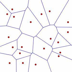
Voronoi diagram.
The downside of these algorithms is that they all suffer from the curse of dimensionality. The space requirement of Voronoi diagrams is $\mathcal{O}(n^D)$, quickly flooding all possible memory capacities. And in high dimensions, querying k-d trees approximates a linear time complexity: $\mathcal{O}(Dn)$.
2.3 Approximate nearest neighbor search with Locality Sensitive Hashing
Due to these impractical complexities, we need to relax the formal definition. Instead of returning a NN, we allow the algorithm to return an approximate NN. The algorithm is allowed to return points, whose distance is at most $cR$ from the query, where $c > 1$ is the approximation factor. The approximate nearest neighbor search algorithm we are interested in is called LSH (Locality Sensitive Hashing). Let’s take a look at the general definition.
We are interested in an LSH family $H$, where for any hash function $h \in H$ chosen at random the following holds:
- if $d(p, q) \le R$, then $P(h(p) = h(q)) \geq P_1$
- if $d(p, q) \gt cR$, then $P(h(p) = h(q)) \leq P_2$
Note that $P_1$ and $P_2$ are not constants, but are varying as $p$ and $q$ change. A given LSH family is only useful when $P_1 > P_2$.
2.3 Hyperparameters
Given a hash function, LSH for NN-search has two hyperparameters.
- $k$: The number of digits of the hash.
- $L$: The number of hash tables initialized with a random hash function.
Given these two parameters, we have the following guarantees for the algorithms (worst case) performance.
- Preprocessing time: $\mathcal{O}(nLkh_t)$, where $h_t$ is the hashing time
- Space requirement: $\mathcal{O}(nL)$, (the data points are stored separately)
- Query time: $\mathcal{O}(L \cdot (kh_t + DnP_2^k))$
With LSH we pay a high price upfront by having a one-time expensive preprocessing operation. In return, we retreive sub-linear query times and reasonable space requirements. Because the preprocessing time is an expensive operation, we don’t want to do a grid search over $L$ and $k$ ($P_1$ and $P_2$ are properties of LSH initialized with $L$ and $k$ and a chosen distance $R$). To reduce optimization time we can let $L$ be dependent on a chosen $k$ and a retrieval probability $P_q$.
The probability $P_q$ of finding a point $p$ within $cR$ is:
$$P_q = P(d(p, q) \leq cR) = 1 - (1 - P_1^k)^L$$
If we solve for $L$ we obtain:
$$ L = \frac{\log(1 - P_q)}{\log(1 - P_1^k)} $$
This enables us to choose a success probability $P_q$ and do a one-dimensional grid search over $k$.
2.4 Euclidean distance
Note that for all hash functions, $h(x)$ is repeated $k$ times with $k$ different random initialized projections to compute the final hash.
Let’s make the LSH algorithm a bit more concrete. Datar et al[2] discussed a hashing function for the L2 distance:
$$ h(x) = \left \lfloor \frac{w^Tx + b}{r} \right \rfloor $$
Where $\lfloor \rfloor$ is the floor operation, $w \sim N(0, I)$, scalar $b \sim \text{Uniform}(0, r)$, and $r$ is a hyperparameter, (E2LSH advises a value of $r=4$ when the data is $R$ normalized).
The collision probability for this hash function is:
$$ P(h(p) = h(q)) = 1 - 2\Phi(-r/R) - \frac{2}{\sqrt{2 \pi} r / R } (1 - e^{r^2/ (2R^2)}) $$
Where $\Phi(\cdot)$ is the CDF of the standard normal distribution.
Note that if we normalize out datapoints $P$ by $\frac{1}{R}$, computing the collision probability with $R=1$ will lead to $P_1$.
2.4.1 Reverse image search
Approximate NN search with L2 distance can, for instance, be utilized with a reverse image search engine. In this example project, I build a reverse image search engine based LSH and the euclidean distance function. When running on the flickr 30k image dataset, we see we can obtain similar colored images choosing an L2 distance with a threshold $R=7000$.

Query image

Collision images
2.5 Cosine similarity
But let’s go to the hashing function we are interested in. We want to obtain a hashing function that represents cosine similarity. Sign Random Projections[3] are such a hashing function.
$$ h(x) = sign(w^Tx) $$
Again, $w \sim N(0, I)$. So $k$ times, a random unit vector is sampled, a dot product is computed and the resulting bit (-1, 1) is stored in the appropriate hash index. Note that the sampling of the unit vectors will only be done once for all hashes.
The collision probability for SRP is:
$$ P(h(p) = h(q)) = 1- \frac{\theta}{\pi}$$
Where $\theta = \cos^{-1} (\frac{x \cdot y}{ \left| \left| x \right | \right | \left| \left| y \right | \right | })$, i.e. the arccos of the cosine similarity between $p$ and $q$.
3 LSH Neural network.
Now that we know how we can make similar vectors collide with high probability. Let’s discuss how we can utilize that in a neural network. The layers of the network need to be hashed and stored (by index) the in LSH tables.
The queries will be the inputs per layer. Per query, only weights of that layer may be returned. It does not make sense to apply weights of the kth to the inputs of the jth layer. For this reason we need to fit LSH tables per layer.
3.1 Forward pass
The figure below shows the steps involved in a forward pass. We only show one layer, as this process is repeated per layer. In the figure below, layer 1, denoted by $x_1^i$, will serve as input for layer 2, denoted by $x_2^i$. The activations of layer 1 are send as a query $q$ to the LSH tables for layer 1. For table $1$ until $L$, the unique hash is determined and the activation neuron id is returned. All the unique neurons are aggregated and returned as activation candidates $a = [x_2^1, x_2^4]$. For these candidates the neuron ouput is computed as $a_i = f(w_i x_i + bi)$. The activated neurons serve as input for the next query to the LSH tables of the next layer. Note that in the next query, the non-activated neuron outputs are zero, resulting in $q = [a_2^1, 0, 0, a_2^4]$.

Layers that sample activations from the LSH tables.
3.2 Backward pass
The backward pass is a bit different than one would implement it in any tensor library. The activated neurons were stored in a buffer and per neuron the gradient was determined by classical message passing, therefore more dealing with objects instead of tensors. It is the same concept as with standard neural networks, it only feels a bit more like bookkeeping when you program it.
3.3 Other
During the training of the network the weights are updated after every batch. That means that the hashes stored in the LSH tables get more and more outdated every update iteration. The writers[1] propose a decaying updating scheme. Where the hashes in the LSH tables get updated in an increasingly delayed time interval. This is needed as updating of the hashes is an expensive opration.
3.4 Implementation in Rust
The above concept is implemented in this project. Here we train a simple feed forward network on the MNIST dataset, yielding the same result with sparse layers as with a fully activated neural network. The code is based on a neural network implementation I wrote earlier in Python + numpy. I’d recommend reading this post if you want a more thorough walk through the code.
The neural network was based on an LSH library I wrote in Rust. You can also create Python bindings for that. So if you ever want fast lookups over millions of rows on data, take a look at this project.
Last words.
Neural networks are becoming increasingly more complex and with that data hungry through the years. The figure below shows the carbon emissions in lbs (cries in metric system!?!) for various models.
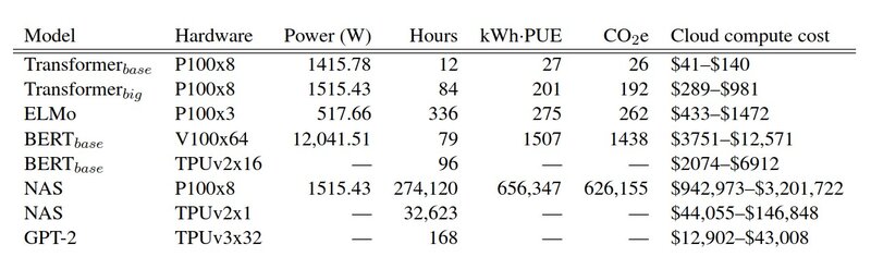
Energy usage models. [4]
Hopefully, the popular tensor libraries, such as pytorch and tensorflow, will add support for this functionality in the future and can deep learning become possible on commodity hardware.
References
[1] Chen & et al. (2019, Mar 7) SLIDE : In Defense of Smart Algorithms over Hardware Acceleration for Large-Scale Deep Learning Systems. Retrieved from https://arxiv.org/abs/1903.03129
[2] Datar, Immorlica, Indyk & Mirrokn. (2004) Locality-sensitive hashing scheme based on p-stable distributions. Retrieved from InSCG, pages 253–262
[3] Moses S. Charikar (2002) Similarity Estimation Techniques from RoundingAlgorithms. Retrieved from https://www.cs.princeton.edu/courses/archive/spr04/cos598B/bib/CharikarEstim.pdf
[4] Strubell, Ganesh, & McCallum (2019, Jun 5) Energy and Policy Considerations for Deep Learning in NLP. Retrieved https://arxiv.org/abs/1906.02243