Soil classification is, in practice, a human process. A geotechnical engineer interprets results from a Cone Penetration Test and comes up with a plausible depiction of the existing soil layers. These interpretations will often be used throughout a project and are input for many following calculations.
Just as the poliovirus, the process of manually mapping data from $x$ to $y$, belongs to the list of things that humanity tries to eradicate from earth.
First few iterations
Automatic soil classification algorithms do exist. The defacto standard is Robertson et al. (1990) Soil Classification Using The Cone Penetration Test. The classifications resulting from their work, often aren’t satisfactory for engineering purposes in the Netherlands. This is due to two reasons.
- The classifications under/ over-represent a certain class (Peat/ Silt)
- Engineers want aggregated layers and the Robertson classifications are per measured layer.
The last point, isn’t criticism of the Robertson classification algorithm, as classification and aggregation are two separate tasks.
If we want to obtain automated classifications that add more value in practice, we need to focus on the points above. So our solution should be able to map input data to a soil distribution and secondly detect changes in the data that represent soil layers.
Data-driven iteration
I believe that a data-driven approach can yield better results than the empirical research-based approach. But to do so we need labeled data. As I don’t have a laboratory nor thousands of hand made labels, I chose to obtain a dataset by querying a database for CPT’s and bore-hole data within 6 meters apart. Any CPT and bore-hole that are less than 6 meters apart are assumed to be from the same soil. The 6 meters cut-of is chosen arbitrarily. The resulting dataset has got flawed labels, but by scraping large quantities of data we hope to approximate the real soil distribution and make the flaws negligible.
For this project, I had roughly 49,000 CPTs and 40,000 boreholes, from which 1,800 pairs met the condition of being less than 6 meters apart.
Cone penetration tests
Cone penetration tests are in situ procedures where a steel bar with a cone is pressed into the ground at a constant speed. During the soil penetration, different things are measured at the cone of the penetration bar.
Shown below is a typical graph resulting from a cone penetration test. Typically two lines are drawn, the qc values and the Fr values. These can be interpreted as
- qc: Resistance measured at the tip of the cone.
- Fs: Friction measured at the cone. The friction is normalized by $\frac{1}{q_c} \cdot 100$, resulting in $R_f$ as these are heavily correlated.
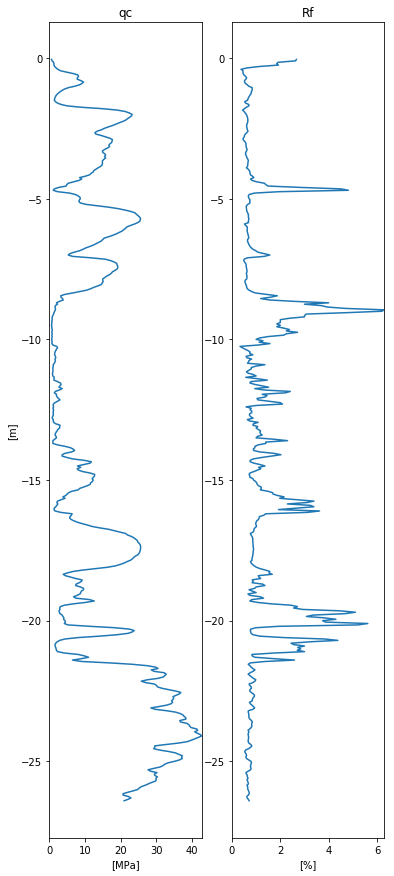
Example cpt
Decision factors
Machine learning is often beneficial with high dimensional data. In this problem, the amount of data dimensions is relatively low. And when training powerful ML models, like Neural Networks (Multi Layer Perceptron architecture) or Gradient Boosting Trees, out of the box on this data, we see comparable results. The results are quite reasonable, but they don’t reflect the decision factor of a geotechnical engineer.
A huge part of the decision making is based on the location where the CPT is taken. And when a CPT, for instance, is taken at sea, they can tell by the curve of the line that a certain layer consists of seashells.
If we want a model to be able to take the same decision factors into account as a human does, it needs to be able to make decision based on the same information.
Model architecture
For this reason, I’ve chosen a Neural Network architecture with convolutional layers that can apply feature extraction on the input signal. Secondly, the model was enhanced with location-based embeddings. This way the model could learn it’s own location embeddings and could learn the probabilities of soil conditional on a certain location. Finally, most of the bore-hole data show that layers concist of multiple volumic parts of soil types. Therefore we should predict the total soil distribution per layer. These adaptations have led to better results than the approaches based on only the qc and Fr values.
Below is shown a result of the model. The model predicts the soil distribution over the depth. Qualitatively the predictions of the model seem very reasonable and align with a geotechnical mapping. Later in the post, we will make a quantitative evaluation.
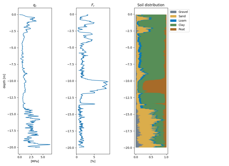
Example prediction
Location embeddings
From the 1800 pairs, 48 location clusters were created by applying K-means on the location data.
In the figure below, the locations of the clusters are mapped on the map of the Netherlands. Sadly the dataset isn’t sufficiently large to fill the entire Netherlands, but it is a good start!
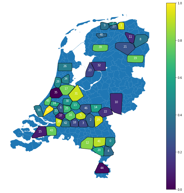
Location clusters
The colors represent a similarity measure between the clusters based on the cosine similarity. Clusters close to each other on the color scale are likely to have similar soil distributions.
Right now the clusters locations and sizes are random. In the future, we could use some domain knowledge to ensure the clusters represent only one soil bias. This is probably beneficial for the model’s results. The cool thing is that the model has learned biases for every location only determined by the dataset. Location 23 and location 32 for instance, are very similar. Which is very likely as both pieces of land are reclaimed from the sea.
Location bias
Besides comparing the clusters by similarity, we can also run inference for the embeddings by nullifying the features. Intuitively this can be regarded as the soil classification you should expect if you don’t know anything, but the location. (This is not entirely true, as the model is not trained on the true distribution due to heavily imbalanced classes.)
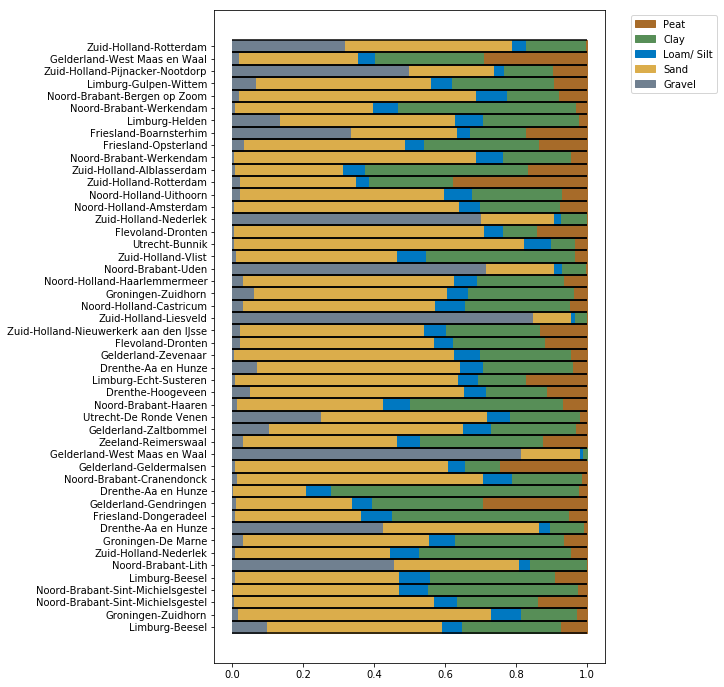
Biases per location
This is quite powerful. During inference, we can decide to use the cluster bias, or if we have our own prior believes about the soil conditions, we could decide to use a different bias.
Metrics
Often when training a machine learning model we have ground truth labels being binary True or False, i.e. $y \in {0, 1}$.

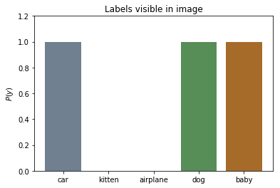
The labels in the image below could, for instance, be a baby, a dog, and a car. In the ground truth labels, we don’t say that the image contains 65% dog, 20% car and 15% baby.
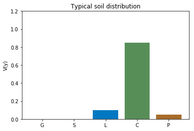
The soil labels are actually distributions. Every layer contains different volumic percentages of soil types, but the sum of all volumes adds up to 1.
Training metric
Cross Entropy
Classification models are often trained by minimizing cross entropy.
$$ H(P, Q) = -\sum_{x \in X} {P(x) \cdot log(Q(x))}$$
In this loss function, it is assumed that that only one index in the ground truth distribution $p=1$, i.e. the labels are one hot encoded. As we’ve just seen, this is not the case for the soil distributions.
Kullback-Leibler divergence
A better metric is the KL-divergence. With this, we actually compare the divergence between two probability distributions.
$$ H(P, Q) = -\sum_{x \in X} {P(x) \cdot log( \frac{Q(x)}{P(x)} )}$$
Wasserstein distance
The best metric I’ve tried for this problem is the Wasserstein distance also being called the Earth mover’s metric. For formality, the definition is shown below.
$$ EMD(P, Q) = \frac{\sum_{i=1}^m \sum_{j=1}^m f_{i,j}d_{i, j}} {\sum_{i=1}^m \sum_{j=1}^n f_{i,j}} $$
where $ D = [d_{i, j}]$ is the distance between $p_i$ and $q_j$, and $F=[f_{i, j}]$ the flow between $p_i$ and $q_j$ that minimizes the overall costs of moving $Q$ to $P$.
$$ \text{min} \sum_{i=1}^m \sum_{j=1}^n f_{i, j} d_{i, j}$$
I’ve actually used the Squared Earth Mover’s Distance-based Loss for Training Deep Neural Networks from Le Hou, Chen-Ping Ye and Dimitris Samaras
This metric makes the most sense in this use case as different soil types have different similarities. This is best explained with an example.
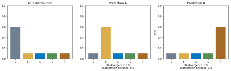
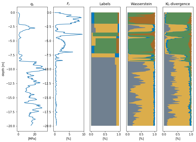
Outcomes of KL-divergence compared to the Wasserstein distance.
In the figure above, we see the outcomes of the KL-divergence and the Wasserstein distance. The KL-divergence only compares the probabilities of the separate classes, but not the shape of the distributions. The KL-divergence outcomes are therefore equal for both predictions. This does not represent what we really want. I believe that assigning volume probability to peat is worse than assigning volume probability to sand when the most volume should be assigned to gravel. By training on the Wasserstein distance we learn the model the order of preference between separate classes.
Validation metrics
Comparing the outputs of the model, optimized by KL-divergence and Wasserstein distance, with Robertson is quite hard. Robertson does not predict a soil distribution, but assigns ambiguous names to soil layers, e.g. ‘Silt mixtures: clayey silt & silty clay’ and ‘Sand mixtures: silty sand & sandy silt’. To be able to make a comparison these, classification were transformed to a soil class $\{G, S, L, C, P\}$.
The bad
A naive way of doing validation is by looking at precision and recall scores by transforming the probability distributions to main soil classes by $\text{argmax}\{P(x)\}$.
F1 scores (higher is better)
| Soil Type | Support | Robertson F1 | KL-divergence F1 | Wasserstein F1 |
|---|---|---|---|---|
| Gravel | 3731 | 0.15 | 0.15 | 0.10 |
| Sand | 137998 | 0.86 | 0.83 | 0.85 |
| Loam | 0 | 0 | 0 | 0 |
| Clay | 91523 | 0.64 | 0.70 | 0.67 |
| Peat | 21398 | 0.37 | 0.57 | 0.74 |
This comparison is of course really bad as we are wasting a lot of information if we reduce a distribution to a number by taking the mode. If we look at the loam soil type, we can clearly see how bad it is. Because loam almost always is a subtype in soil layers it will never come out as the main soil, making it look that no model can predict this class.
The good
Below we show the error distributions. Because we are talking about probabilities, these distributions show us our error margins. In the plots, we also show the Mean Absolute Error (MAE), per soil type, so we can make a proper comparison. We show the absolute errors on two subsets of the test set.
- A subset where the true distribution has non zero probability for that class. Can intuitively be regarded as recall.
- A subset where the models assigns a significant probability to that class $P(y) \gt 0.025$. Can intuitively be regarded as precision.
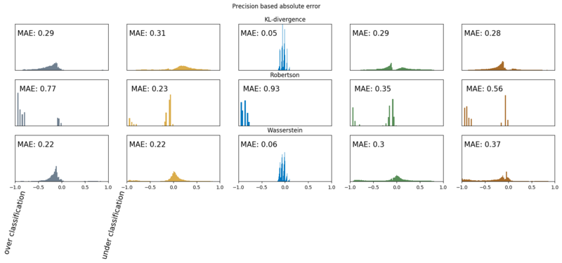
Precision based absolute errors (lower is better)
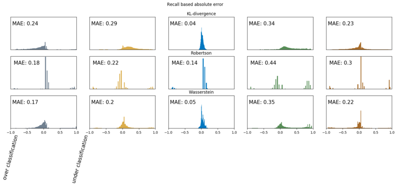
Recall based absolute errors
Now we can clearly see how the models are performing. When looking at the precision based results, we, for instance, see that most of Robertson’s loam and gravel classifications are wrong, and for peat, a classifcation is wrong ~50% of the time. Due to this sensitivity to Loam, Robertson’s recall based error is much lower. Further, we see, that the KL-divergence model does best for the soil types loam, clay, and peat. For the soil types gravel and sand, the Wasserstein model shows the least errors and has a slightly lower error rate for peat at the recall subset. These plots are way more informative than the main soil based f1 scores. We do see that both models outperform Robertson on the soil classification task.
Grouping
The second challenge was creating aggregated layers. Engineers don’t want too small layers in there FEM software, as that messes up the mesh. And often they’d need to write a report on the soil conditions and don’t feel much for reporting my output of ~750 soil layers.
Gaussian signal
For the grouping, we assume the cpt signal $X_t$ coming from a Gaussian distribution.
$$ X_t| \mu, \sigma \sim N(\mu, \sigma)$$
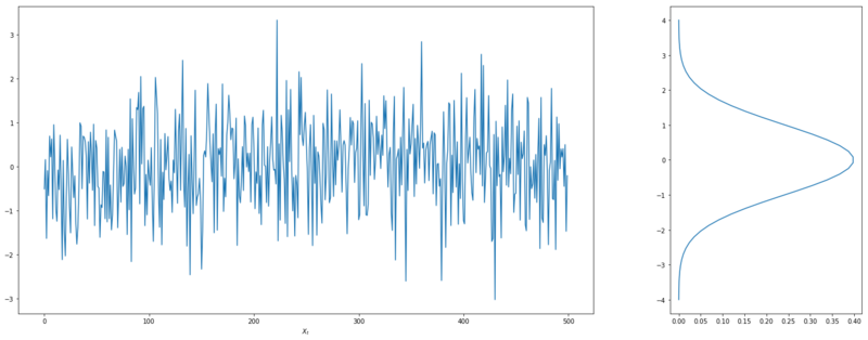
Gaussian signal
Now the likelihood of this signal is determined by
$$ \mathcal{L}(X_t, \mu, \sigma) = \prod_{t=1}^{n}P(x_t | \mu, \sigma)$$
Changepoint
Now we assume the signal below. The likelihood of those signals coming from two Gaussians, separated by changepoint $\tau$, is higher than the likelihood of the whole signal coming from one Gaussian.
$$ [\mathcal{L}(x_{1:\tau}) + \mathcal{L}(x_{\tau:n})] > \mathcal{L}(x_{1:n}) $$
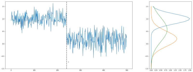
Two Gaussian signals with changepoint $\tau$
Optimization problem
This observation can be turned into an optimization problem. We search for the minimal negative likelihood by adding new changepoints $\tau_i$ for every point $k$ in the signal. To prevent having changepoints at every data point, we introduce a penalty $\lambda$.
$$ \min_{k, \tau}{ \sum_{i=1}^{k+1}[-\mathcal{L}(x_{\tau_{i-1} : \tau_i})] + \lambda } $$
Final results
Below we see some inference results on the test data.
Below it is also clearly visible that the dataset contains flawed labels. Both models correctly identify the sand layer, where the labels show (wrongly) otherwise.
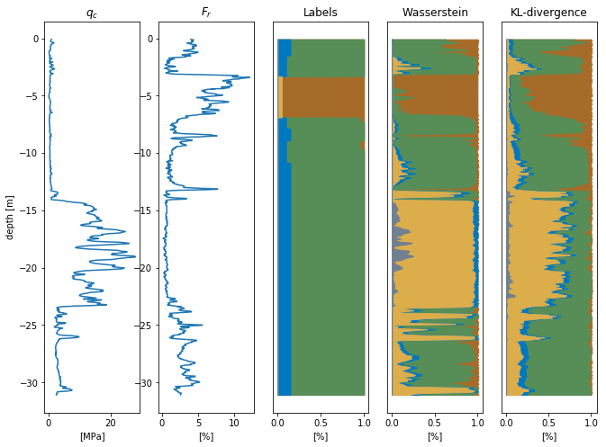
Prediction where the test set is wrongly labeled.
And finally, an example of the predictions with grouping applied. The cool thing is we can tweak the grouping algorithm. By nudging $\lambda$ we can choose to have more layers (and have more information) or group more with fewer layers as a result. The grouping prediction below is made with the Wasserstein based model.
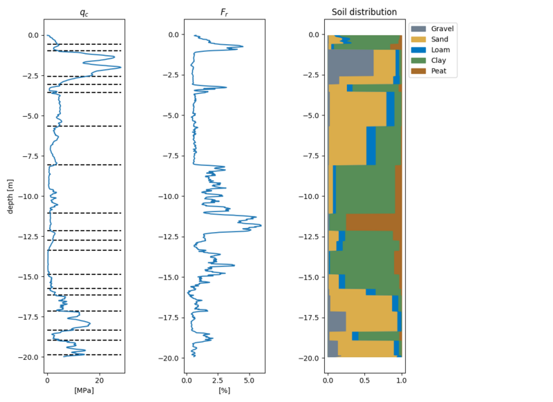
Prediction with grouping applied.
Last words
This model has been in the pipeline for quite some long time. I’ve been working on it on and off. Every now and then I had an idea, and tried it with renewed energy. At the moment I’m helping CruxBV with their quest to automation. As a geotechnical firm, they really are benefited by automated soil classification. This encouraged me to finish the work I’ve done on the model and put it in production in their landscape.