This post continues where part 2 ended. The Runga Kutta algorithm described in last post is only able to solve first order differential equations.
The differential equation (de) for a single mass spring vibrations problem is a second order de.
Note that in this equation:
u’’ = acceleration a
u’ = velocity v
u = displacement
Before we can solve it with a Runga Kutta algorithm we must rewrite the base equation to a system of two first order ode’s.
Rewrite:
Now there a set of coupled ode’s. Both need to be solved together. The solution of both ode’s is determined by:
Where v1 - v4 and a1 - a4 are determined as described in the table below. Note that:
| Column values | t | u | v | a |
|---|---|---|---|---|
| t1, u1, v1, a1 | ti | ti | vi | f(t1, u1, v1) |
| t2, u2, v2, a2 | ti + h/2 | ti + v1h/2 | vi + a1h/2 | f(t2, u2, v2) |
| t3, u3, v3, a3 | ti + h/2 | ti + v2h/2 | vi + a2h/2 | f(t3, u3, v3) |
| t4, u4, v4, a4 | ti + h | ti + v3h | vi + a3h | f(t4, u4, v4) |
Code
If we make this in python we get the function below. The input is an array with time values; t. We set the displacement and velocity at the first value of the times array. Furthermore we pass the mass, the damping and the spring stiffness of the system.
def runga_kutta_vibrations(t, u0, v0, m, c, k, force):
    """
    :param t: (list/ array)
    :param u0: (flt)u at t[0]
    :param v0: (flt) v at t[0].
    :param m:(flt) Mass.
    :param c: (flt) Damping.
    :param k: (flt) Spring stiffness.
    :param force: (list/ array) Force acting on the system.
    :return: (tpl) (displacement u, velocity v)
    """

    u = np.zeros(t.shape)
    v = np.zeros(t.shape)
    u[0] = u0
    v[0] = v0
    dt = t[1] - t[0]

    # Returns the acceleration a
    def func(u, V, force):
        return (force - c * V - k * u) / m

    for i in range(t.size - 1):
        # F at time step t / 2
        f_t_05 = (force[i + 1] - force[i]) / 2 + force[i]

        u1 = u[i]
        v1 = v[i]
        a1 = func(u1, v1, force[i])
        u2 = u[i] + v1 * dt / 2
        v2 = v[i] + a1 * dt / 2
        a2 = func(u2, v2, f_t_05)
        u3 = u[i] + v2 * dt / 2
        v3 = v[i] + a2 * dt / 2
        a3 = func(u3, v3, f_t_05)
        u4 = u[i] + v3 * dt
        v4 = v[i] + a3 * dt
        a4 = func(u4, v4, force[i + 1])
        u[i + 1] = u[i] + dt / 6 * (v1 + 2 * v2 + 2 * v3 + v4)
        v[i + 1] = v[i] + dt / 6 * (a1 + 2 * a2 + 2 * a3 + a4)

    return u, v
Lets say we have got a mass spring system with the following parameters:
- Mass m = 10 kg
- Stiffness k = 50 N/m
- Viscous damping c = 5 Ns/m
On this system we are going to apply a short pulse. The force on the system is described by the following array:
n = 1000
t = np.linspace(0, 10, n)
force = np.zeros(n)

for i in range(100, 150):
    a = np.pi / 50 * (i - 100)
    force[i] = np.sin(a)
It is an array of zeros for most of the time values t. Only a small part off the array will be a peak. Now we are going to define the parameters of the system, call the runga_kutta_vibrations function and plot the result together with the force.
# Parameters of the mass spring system
m = 10
k = 50
c = 5

u, v = runga_kutta_vibrations(t, 0, 0, m, c, k, force)

# Plot the result
fig, ax1 = plt.subplots()
l1 = ax1.plot(t, v, color='b', label="displacement")
ax2 = ax1.twinx()
l2 = ax2.plot(t, force, color='r', label="force")

lines = l1 + l2
plt.legend(lines, [l.get_label() for l in lines])
plt.show()
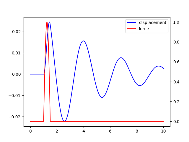
Vibration resulting from a pulse.
If we look at the plot figure. We can see that before the pulse is acting on the system the amplitude is zero. There is no force acting on the system and therefore there is no oscillation. At approximately 1 s, a short puls acts on the system and the system responds. The rest of the plot shows the system oscillating in its natural frequency.
As you can see, we now can describe a vibrations problem of a singe degree of freedom system nummerically. The Runga Kutta method can be used with predefined force functions as we did (We described the pulse with a sine function, but it can also be used with vibration data resulting from measurements.